Challenges when Creating Variable-structure Models

Alexandra Mehlhase, Daniel Gomez Esperon and Thomas Karbe

Software Engineering, Technische Universit

at Berlin, Ernst-Reuter-Platz 7, 10587, Berlin, Germany

Keywords:

Variable-structure models, Mathematical models, Differential equations, Modeling guidelines.

Abstract:

Variable-structure models can switch their system of equations during a simulation, allowing for a change

of level of detail or behavior. The need for this kind of models has been well-established, and there are

simulation environments that can handle them. While most research papers on this topic focus on language

and tool issues regarding variable-structure models, in this paper, we will shed some light on the pragmatics

of actually creating such a model in a reusable way. During the construction of a variable-structure model, the

modeler will face several challenges, such as the initialization of new modes during mode switches. We will

collect and discuss the most important challenges and, if possible, provide rules of thumb on how to handle

these challenges appropriately.

1 INTRODUCTION

According to Mahr, modeling means always to create

a model of something for some purpose (Mahr, 2008).

Thus, on the one hand, a model is always an abstract

representation of some other entity. Only some of its

properties are taken over to the model, while others

are left out on purpose. On the other hand, the se-

lection of those properties is guided by the purpose

of the model. In (Top, 1993) the author gives a more

speciﬁc explanation:

The modeling problem is to construct the most

simple artifact that allows an adequate answer

to a given query.

Therefore, the quality of a model could be judged by

the simplicity of the model, as long as it fulﬁlls its

purpose.

This means that the main challenge in modeling is

to ﬁnd the right level of abstraction to answer a given

query. It should not include any information that is

not necessary for the answer, but all information that

is needed.

In the ﬁeld of mathematical models with

differential-algebraic equations (DAEs), there are two

major factors that add complexity to the modeling

problem. First, models tend to become quite large and

are therefore split into submodels, which are models

on their own for some part of the problem domain

which can be reused. Second, during the course of a

simulation sometimes different aspects of the problem

are of interest or needed in a different level of detail.

An example of this is the model of an airplane

taking off on a runway, then increasing height, and

ﬁnally arriving at traveling height. Since in this ex-

ample three different stages of a ﬂight are simulated,

there should be three speciﬁc models, one for each

stage. Then, the ﬂight simulation should switch be-

tween the different models when appropriate.

Models with different states between which they

can switch during simulation depending on the cur-

rent situation are called variable-structure models.

Each state in such a model is called a mode, and the

model can switch between modes through transitions.

While simulating such a model one mode is always

active and represents a state of the modeled system.

When a transition is activated through a guard, a new

mode becomes active. The new mode then needs to

be initialized and the simulation continues in the new

mode.

It is well-established that there is a need for

variable-structure models and that they can gener-

ally be handled in a simulation environment (Heinzl

et al., 2012), (Elmqvist et al., 1993). However, these

environments are mostly prototypes or experimental

frameworks for now. In these specialized frameworks

the models need to be reimplemented in the language

speciﬁc to the framework. Common simulation envi-

ronments like Dymola (Dassault Systems, 2015) and

Simulink (The MathWorks Inc., 2013a) provide only

limited support of variable-structure models.

Therefore, there is not much experience with mod-

eling large models or how to adapt models, which al-

101

Mehlhase A., Gomez Esperon D. and Karbe T..

Challenges when Creating Variable-structure Models.

DOI: 10.5220/0005521601010110

In Proceedings of the 5th International Conference on Simulation and Modeling Methodologies, Technologies and Applications (SIMULTECH-2015),

pages 101-110

ISBN: 978-989-758-120-5

 2015 SCITEPRESS (Science and Technology Publications, Lda.)

ready exist, in simulation environments like Dymola

or Simulink. Using modes and transitions between

modes gives modelers a much wider tool set, but it

also introduces new challenges that have to be con-

sidered. In non-variable-structure models, the mod-

eler just had to ﬁnd appropriate start values for the

one model. Now, he also has to decide when and

how often a mode switch should take place, and for

each mode switch, how to initialize the newly acti-

vated mode.

In this paper, we regard modeling of variable-

structure models, since it is already shown in differ-

ent papers that variable-structure models can be sim-

ulated. We present a collection of challenges that

often occur when creating variable-structure models,

and give rules of thumb (RoT) to handle them. These

challenges and ruled of thumb are regarded indepen-

dent of the domain and hold true for models which are

described with differential-algebraic equations.

Chapter 2 gives a basic overview of the state of

the art in variable-structure modeling and simulation.

Chapter 3 covers the architecture of variable-structure

models regarding their equations, variables and inter-

faces. In Chapter 4 the initialization routines are dis-

cussed in detail while Chapter 5 focuses on guards of

transitions. Chapter 6 summarizes the evaluation of

the proposed rules of thumb. Chapter 7 concludes

the paper and presents future works.

2 STATE OF THE ART

General purpose modeling languages like Modelica

(by the Modelica Association (The Modelica Asso-

ciation, 2012)) and Matlab Simulink are well estab-

lished but their support for variable-structure models

is very limited. This special form of modeling has

been investigated for more than twenty years (Heinzl

et al., 2012). Many different experimental languages

and simulation environments have been developed to

model and simulate changes in model structure.

One of these tools is MOSILAB (Nytsch-Geusen

et al., 2005), (GENSIM Project, 2007), which uses

a Modelica-like language to describe the models.

The modes and transitions are described through a

Statecharts-like (Harel, 1987) view. The simulation

is realized through an integrated simulation engine.

In MOSILAB only Index-0 models can be simulated

since no index-reduction is integrated yet.

Another approach is the experimental language

SOL which provides a language and a simulator (Zim-

mer, 2010). The variable-structure simulation frame-

work of SOL can handle higher-index models.

Another tool often used is Ptolemy (Ptolemaeus,

2014) which also enables the modeler to use different

modes.

Other approaches to describe variable-structure

models in speciﬁc languages are the theorem prover

for hybrid systems called KeYmaera (Platzer and

Quesel, 2008), the functional language Hydra (Nils-

son et al., 2003), the event based approach of DEVS

(Pawletta et al., 2002), the Matlab/Simulink libraries

SimEvents (Clune et al., 2006), and Stateﬂow (The

MathWorks Inc., 2013b).

A framework to model and simulate variable-

structure models without having to implement the

modes in a new language is introduced in (Mehlhase,

2013). Here, common simulation environments are

used to simulate each mode whilst the mode changes

are handled by the framework.

The current state of the art is that variable-

structure models can be modeled and simulated.

There are algorithms, tools and frameworks to sim-

ulate and test such models. A formalization ap-

proach to tackle challenges of hybrid systems, to

which variable-structure models belong, is described

in (Mosterman and Biswas, 1997).

Yet, it is not well-established what has to be con-

sidered and what challenges occur compared to clas-

sical modeling.

3 BASIC ARCHITECTURE OF

VARIABLE-STRUCTURE

MODELS

It is important to understand the principles and goals

in classical modeling before discussing the challenges

of variable-structure modeling in detail.

A real system usually consists of many related

components. Each of these components is also a sys-

tem and can consist of components itself. It is there-

fore built hierarchically. This approach is necessary

to be able to build systems out of components and ex-

change components if necessary.

While modeling such a system it is helpful to use

the same approach and create a model that has com-

ponents which can again consist of components. A

model that describes a part of a whole will be called

component. Components on one hierarchy level can

be connected through the variables in their interfaces.

An interface is a collection of variables and compo-

nents can have an arbitrary number of interfaces. Fig-

ure 1 shows three components (A, B, C) connected

through their interfaces (circles appended to the com-

ponents). These interfaces are connected through

equations (rectangles on connecting line) which de-

SIMULTECH2015-5thInternationalConferenceonSimulationandModelingMethodologies,Technologiesand

Applications

102

scribe the relation between these interfaces. We will

call these equations relation-equations to not confuse

them with Modelica connect-equations since they do

not have the same semantics. The relation-equations

can be any kind of equation to specify the connec-

tion of interfaces. Therefore, the relation-equations

are a more general description and abstract the Mod-

elica connect-equations as well as Simulink connec-

tions between interfaces.

B C

}

= f (b

)

}

= c

}

, b

}

= 2 ∗c

= c

}

Figure 1: Model with three components.

Each component encapsulates behavior and

should be usable in different contexts. A created com-

ponent can therefore be used many times as long as

the interfaces of the component can be connected.

When looking at variable-structure models, the

exchange of components itself needs to be mod-

eled. Therefore, it is sensible to encapsulate such ex-

changes in components to enable reusability.

3.1 Modes and Transitions

A variable-structure model generally consists of an ar-

bitrary number of modes. A mode is a component

which can be exchanged during simulation through

another component.

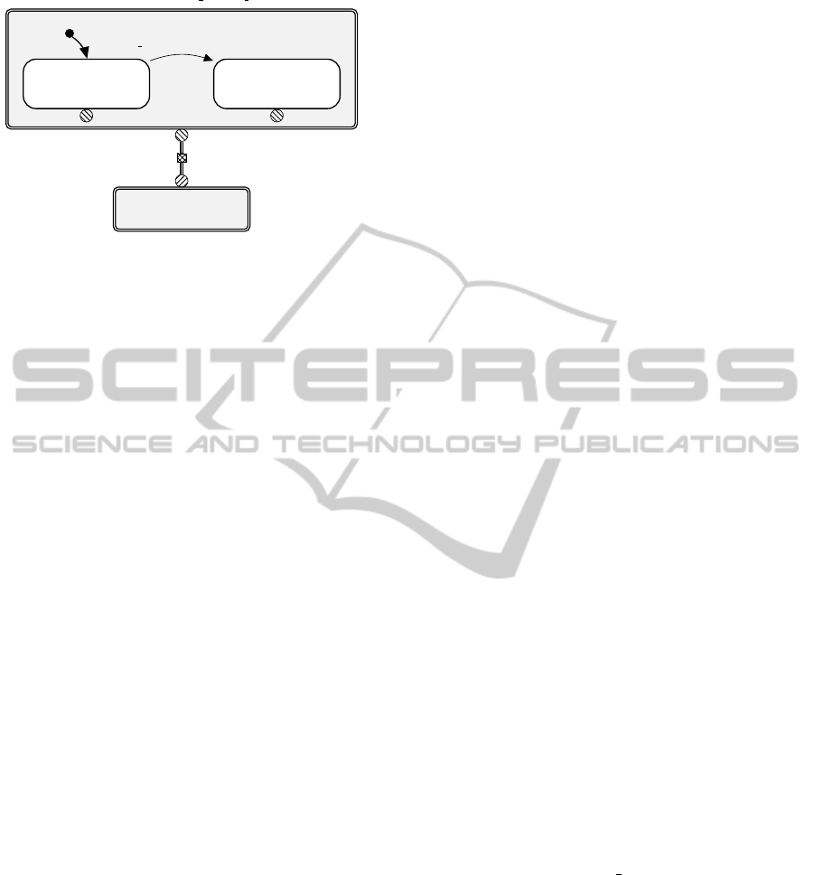
Figure 2 shows a simple variable-structure model

in a Statecharts-like syntax. The model consists of

four modes (A, B, C and D) and is always represented

by one of them.

Like in Statecharts an initial mode has to be de-

ﬁned. Furthermore, the ﬁrst mode might need to be

initialized with user-deﬁned values. This initializa-

tion process is equivalent in classical modeling. In

this example mode A is the initial mode and is initial-

ized through init.

Each transition leads from one mode to another.

A transition is activated when a guard (e.g. a1

, b1

)

becomes true. When a transition is activated, the sim-

ulation of a mode stops and the new mode needs to

be identiﬁed. This new mode needs to be initialized

through a routine deﬁned in the transition. During the

mode switch the simulation time does not continue.

A B

⇒ B1

⇒ B2

⇒ D

⇒ A2

⇒ A1

⇒ C

⇒ B3

init

Figure 2: Variable-structure model with four modes.

Simulation time only moves on during the simulation

of a mode.

A transition therefore consists of the following in-

formation:

• Pre mode

• Post mode

• Guard

• Initialization routine.

3.2 Modes in Components

So far we have looked at components and their rela-

tion and modes in general. Now we take a look at

modes inside a component. Models usually consist of

components which can often be used in other mod-

els. Many modeling tools/languages (e.g. Modelica)

have libraries with components. These can be used to

create a speciﬁc model. The same should be possible

with components containing modes. To accomplish

this the modes and components have to fulﬁll certain

criteria.

3.2.1 Interfaces

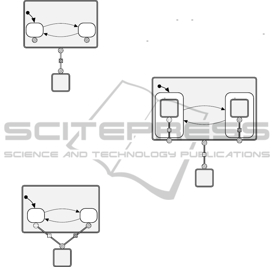
Figure 3 shows a model with two components.

Component A has two modes, therefore it is repre-

sented by either the component A1 or A2 at a speciﬁc

simulation time. If the interfaces of A1 and A2 are

identical, the relation-equations to the component B

do not have to change during a mode switch.

Only the intern variables and equations of A

change.

RoT-1 uniform interface I: For reusable compo-

nents all modes in the component should have the

same interfaces.

ChallengeswhenCreatingVariable-structureModels

103

A1 A2

⇒ A2

⇒ A1

init

Figure 3: Component A consists of two modes with identi-

cal interfaces.

When this model is simulated, it starts with the

compositions of A1 and B since A1 is the initial mode

of A. When the transition is activated, the component

A2 is initialized and the simulation of the composition

of A and B is resumed.

If the interfaces of the modes are not identical, the

mode switch is not as simple. The mode switch can-

not be deﬁned locally since the relation-equations to

the other components also need to change.

A1 A2

⇒ A2

⇒ A1

init

Figure 4: Model with two components. Component A has

two modes with different interfaces.

Figure 4 shows such an example. Such a model

can be created but the advantage of reusability is lost

since component A with its modes cannot be used in

other models without adapting the context the com-

ponent is used in. In Figure 4 the relation-equations

are different for the two modes, represented through

the two separate connecting lines. The goal is to cre-

ate components with modes which can be used in

different models the same way a component without

modes can be used.

The interfaces of the modes should be adapted

to be the same in all modes. Adapting the inter-

faces is straight forward since the individual relation-

equations of the modes can be used to deﬁne the new

interface which then matches the needed one. Fig-

ure 5 shows this approach graphically. New modes

are created (A1 a, A2 a) that wrap the old modes (A1,

A2) to adapt the interfaces. The old modes (A1, A2)

are then only components and the new modes (A1 a,

A2 a) consist of the old mode and the old relation-

equation with the new interface.

The mode switch is again local inside a compo-

nent and Component B needs no information about

the mode switch.

A1 a A2 a

A1 A2

⇒ A2

⇒ A1

init

Figure 5: Model with adapted interfaces.

RoT-2 uniform interface II: If modes in compo-

nents do not have the same interface, the modes

should be encapsulated by an adapter mode.

3.2.2 Variables and Equations Inside Modes

The different combinations of active modes with other

components must lead to a solvable system of equa-

tions. In Figure 4, this means the composition of A1

and B as well as A2 and B must be a solvable system

of equations.

RoT-3 solvable combinations I: All reachable mode

combinations must lead to a solvable system of

equations.

For the simulation in current environments it is a

necessary requirement that the number of equations

and number of unknown variables in a model are

equal. As presented in (Broman, 2010) one can depict

a Constrained Delta C

∆

for each component. This C

∆

represents the delta of equations to unknown variables

for each component. A model can only be simulated

if the C

∆

is zero. Otherwise the system of equations

is not solvable. In a component consisting of com-

ponents the relation-equations as well as the variables

SIMULTECH2015-5thInternationalConferenceonSimulationandModelingMethodologies,Technologiesand

Applications

104

and equation of each component are taken into ac-

count.

To deﬁne encapsulated components with modes

the C

∆

has to be the same in all modes. Otherwise the

modes are not locally exchangeable since the overall

∆

would differ from zero if the context of the com-

ponent does not change during a local mode switch.

RoT-4 solvable combinations II: All modes in a

component must have the same C

∆

for locally de-

ﬁnable mode switches.

4 INITIALIZATION

To understand the importance of a correct initializa-

tion it is necessary to look at the basics ﬁrst. The ini-

tialization of a set of differential-algebraic equations

inﬂuences the results and sometimes even the stability

of the simulation’s results signiﬁcantly.

A steady-state is often sought after for the initial-

ization to minimize the possibility of wrong results

(Casella et al., 2011).

When regarding variable-structure models it is not

only necessary to ﬁnd a consistent set of values for the

start of the simulation. Instead, for each mode switch

a separate initialization needs to take place. This ini-

tialization mostly depends on the state the model was

in when the transition was activated and it is not suf-

ﬁcient to use static values. The initialization routine

is part of the transition since only the transition has

information about the previous and the next mode.

RoT-5 initialization: Each transition must deﬁne

an initialization routine.

4.1 Using the Last State of the Old

Mode

The easiest way to initialize a mode is by starting

the simulation where the old mode left off. An ex-

ample of this is a pendulum (mode 1) becoming a

falling mass (mode 2) when the centrifugal force is

smaller than zero. In this case the simulation of the

falling mass should start at the exact position and ve-

locity where the pendulum simulation left off. As-

suming both modes have the necessary variables x,

y, vx and vy representing the position and velocity, a

simple one-to-one-mapping is possible that maps the

old state to the new state.

If the modes of a transition do not have the same

variables, such a one-to-one-mapping of values is not

possible. For the above example the pendulum mode

might only have the variables for the angle ϕ and the

angular velocity der ϕ. The falling mass on the other

hand needs the Cartesian coordinates. In this scenario

a calculation needs to take place to transform the old

state to the new state (mapping).

RoT-6 initialization Function: The initialization

can use the previously simulated data of the old

mode to initialize the next mode through a map-

ping.

4.2 Using Past Data

In variable-structure models it is not only possible to

exchange components but also to delete or generate

new components. In case an added component has

not previously been in the model it might not be sufﬁ-

cient to use only the previously calculated simulation

results. An example of such a model is a pipe net-

work where some of the pipes where cut off through

valves at the beginning of the simulation. When a

valve opens, further pipes need to be simulated. The

modeler has to give information about the state the

new pipe or pipes should be in after a transition.

RoT-7 component Generation: The initialization

can use external data.

Another scenario might be that a pipe gets cut off,

which enforces a mode switch and later on the pipe is

added again. In such a case it can be sensible to use

the old state of the pipe for its initialization. Meaning

that not only the past data of the previous mode is

necessary in the initialization routine but also the past

data of this mode’s own previous state.

RoT-8 state Storage: The initialization has access

to previous states of the new mode.

4.3 Time Consuming Transitions

Transitions also require modeling since they describe

the whole switching process from one mode to an-

other. This model did for now not need any simu-

lation time and was not simulated by a solver. The

simulation of the previous mode stopped and so did

the simulation time until the next mode’s simulation

was started.

Sometimes such an abrupt change is not feasible

and leads to discontinuities in the simulation’s results,

which should usually be avoided. Therefore, transi-

tions can be modeled with their own mode. Mean-

ing that for a desired switch from A to B there ex-

ists a third mode AB which models the transition. Of

course, then there need to be transitions from A − AB

and AB − B but since the mode AB is created merely

ChallengeswhenCreatingVariable-structureModels

105

for the transition from A to B the two transitions can

usually be kept quite simple.

Two different kinds of in-between modes are pos-

sible:

1. Deriving the in-between Mode from the modes

A and B: An in-between mode can be derived

by simulating both modes simultaneously. Dur-

ing the simulation of the in-between mode results

of the two modes are weighted. The simulation

is started with the old mode weighted with 100%

and the new mode with 0% and altered until the

old mode has a weight of 0% and the new one of

100%. The mode switch should then not have any

discontinuities in the important variable’s values.

This approach is possible when the level of detail

is changed. If the behavior changes, it is usually

not the case that during a switching period both

modes are valid. A drawback of this method is

that during the mode switch two systems of equa-

tions are used, which makes the simulated system

of equations quite large.

2. Creating a new in-between Mode: A new mode

can be deﬁned that models the mode switch with

equations exclusively for this mode switch. This

is for instance useful for clutches. In one mode

the clutch is disengaged in the other one engaged.

The transition is neither possible to model with

the one or the other mode since the clutch is some-

where in between.

This approach is possible when there is a switch

in behavior. Usually this means that more modes

need to be regarded than were obvious.

RoT-9 Time Consuming Transitions: For complex

transitions an in-between mode should be intro-

duced.

4.4 Jump Into the Past

The above initializations assumed that the simula-

tion of the next mode starts where the old simula-

tion stopped. Sometimes, it is necessary that the new

mode’s simulation does not start exactly where the old

simulation left off. If the current mode is less detailed,

the deviation that causes the transition event might be

detected too late. In such a case it is useful to go back

in time during a mode switch to let the new mode’s

simulation start off at a time step when the result was

more accurate. Then, a critical point can be calculated

anew to make certain that the values are correct. Fur-

thermore, it allows to calculate the new start values in

a region when the old mode is still in a state where it

was valid, e.g. steady-state.

Figure 6 shows how the results of such a simula-

tion might look like. It is assumed that a less detailed

mode is used with a variable x. The delta between

the values of x from two time steps is used to acti-

vate a transition. Since the mode is assumed to be

less detailed, the variable might not change as fast as

it would in a more detailed mode. When the transition

is activated there is a time jump into the past and the

more detailed mode is initialized with past data.

Time

Jump

less detailed

detailed

∆x

Figure 6: Mode switch with a jump into the past

Here the modeler has to decide how far the sim-

ulation time should be reset. For the speciﬁed time,

initialization values need to be available.

RoT-10 past states: The initialization has access to

past states to allow for steps back in time.

4.5 Initialization for Modes in

Components

The approaches above regarded the initialization in

general and they are valid for transitions on the high-

est hierarchy level and on the component level.

When looking at the component level, the scope of

the components has to be considered. Since the idea

of a component is to encapsulate behavior, a compo-

nent can only use data available in this component.

This applies to modes in a component as well as to

the transitions between these modes.

Consider Figure 7 which presents a model with

two components. One component represents a pipe

which is split into 100 elements to calculate the mass

(m), pressure (p) and temperature (T) accurately. The

other mode only has 10 elements and is less detailed.

This gives us the means to calculate the values of the

above variables more or less accurately during the

simulation. The pipe is connected on one side to a

throttle which calculates a mass ﬂow out of the pipe

depending on the temperature and pressure from the

pipe’s end and a parameter P. The pressure and tem-

perature are assumed to be inputs for the throttle while

the mass ﬂow is the output.

SIMULTECH2015-5thInternationalConferenceonSimulationandModelingMethodologies,Technologiesand

Applications

106

Pipe

Pipe detailed

elements = 100

Pipe simple

elements = 10

extend transition(t id): init new

t id: guard ⇒ init

init

Throttle

m f low = f (p, T, P)

p, T , m f low

p, T , m f low p, T , m f low

Figure 7: Pipe model with components Pipe and Throttle.

The initial state of the model is the pipe with 100

elements connected with the throttle. When a mode

switch occurs, for instance because the temperatures

in the elements do not differ much anymore, the new

mode with only 10 elements needs to be initialized.

In this case it is sensible to combine 10 elements into

one new element, e.g. t1

new

= mean(t1

old

, . . .t10

old

new

= sum(m1

old

, . . . , m10

old

During a mode switch as described above the val-

ues of T and p change during the initialization rou-

tine. When the pressure and temperature change, the

mass ﬂow through the throttle also has to change since

it depends on T and p. The local mode switch in the

pipe implicitly changes a value of the throttle. This

also means that the switch is not local. As soon as

output variables (p, T ) change their values and inﬂu-

ence connected components, the initialization is not

restricted to the component the mode switch is in.

To make sure that this does not occur one should

abstain from changing output values during a local

mode switch. This might of course be difﬁcult to en-

sure in acausal modeling since during the modeling of

the components the outputs are not deﬁned and are de-

pendent on the context. In a modeling language with

causal behavior this is easier to realize since the in-

put/output relation is hard coded.

RoT-11 change of outputs: The initialization in a

component should not change output values.

Since the above rule cannot be ensured all the

time, there need to be possibilities and rules to han-

dle initialization routines implicitly to change values

from other components. There are different possibili-

ties which can be assumed during such mode switches

in components:

1. Everything not speciﬁed should stay the same.

This means that only the values of the variables

in the switching component are inﬂuenced. All

other components without a mode switch try to

keep their values. This usually means that the pa-

rameters and state variables will keep their values

whereas other variables might change their values,

e.g. mass f low changes while P keeps its value

even though this leads to a discontinuity in the

mass ﬂow.

2. Everything not speciﬁed must stay the same:

This means that all variables and parameters from

components without a mode switch must keep

their values. Therefore, it would not be allowed

to change the values of output variables during an

initialization routine. If all outputs keep their val-

ues, values of other components do not have to

change.

3. Local transitions know the global context: This

means that transitions have access to the con-

text they are in and can therefore initialize other

components. This is often an approach in state

machines and their parallel components (Harel,

1987). In the context of modeling this does not

seem feasible since the context of a component

should be exchangeable and a component should

have a local scope. Otherwise it would not be pos-

sible to use a component with modes in different

contexts.

4. Extension of local transitions: This means that

the user can extend or redeﬁne local transitions in

one of the higher hierarchy levels if necessary. In

most cases it should sufﬁce to use the local transi-

tions but sometimes it is not possible to initialize

the new mode and its context correctly through

the local initialization routine. If this is the case,

it should be possible to overwrite the local transi-

tion on a higher hierarchy level and redeﬁne the

initialization routine. To accomplish this a tran-

sition should have an ID. This ID can be used to

identify the transition to be overwritten. Since this

new routine is on a higher hierarchy level, it can

use data from its current hierarchy level and is not

limited to the local scope of the old transition.

In the example above such an extended transition

is used to overwrite the initialization routine of

the local mode with init new. In this routine one

might deﬁne that the value P should change rather

than the value of m f low to avoid discontinuities.

We suggest a mix of the ﬁrst and fourth approach.

When nothing else is speciﬁed the values of parame-

ters and state variables should keep their values. But

to make the initialization more ﬂexible the modeler

should have the means to overwrite or extend a transi-

tion to specify a global initialization which takes the

variables of other components into account.

RoT-12 change of Outputs: The initialization can

be extended on a higher level.

ChallengeswhenCreatingVariable-structureModels

107

5 GUARDS

A transition is activated when its guard becomes true.

During its activation the transition leads to a mode

switch which uses the initialization routines already

discussed. As a result of the modularization and the

local scope of components the guards of transitions

inside of components can only depend on the local

data of that component’s currently simulated mode.

Otherwise the components would again not be ex-

changeable since it would be context dependent.

5.1 Basics

The most basic decision regarding transitions is when

a mode switch should occur. In some cases this is sim-

ple as with the already discussed pendulum example.

When the centrifugal force (F

centri

) is below zero the

mass of the pendulum will not continue on its circular

path. The mass will begin to fall which leads to dif-

ferent equations to describe the behavior. The guard

would therefore be F

centri

< 0.

When looking at changes in the behavior it is often

possible to look at the real system and fragment the

behavior in different phases depending on the mathe-

matical description which is necessary for the differ-

ent phases. If two phases of a real system do not need

different sets of equations to describe their behavior,

there do not need to be two modes in a mathematical

model. If the phases are obvious, it is often possible

to ﬁnd obvious guards when to switch. It is important

though that the guards are chosen in a manner that

avoids many switches back and forth between two

modes in a short time (also called chattering). This

can be avoided by using hysteresis in the guards or by

demanding that a mode is active for a minimum time.

RoT-13 avoid chattering: Chattering between two

modes should be avoided.

Regarding variable-structure models which switch

their level of detail, the guard is usually not clear since

both modes describe basically the same system only

with a different granularity. The modeler has to de-

cide when the switch of detail needs to take place.

The modeler already decided about the granularity of

the modes when he created them and probably has a

basic idea why and when this switch should occur. As

was shown and discussed in Figure 6 the choice of the

guard can inﬂuence the simulation signiﬁcantly.

When in doubt the modeler should use the more

detailed mode for longer periods than necessary in-

stead of switching too early. If the results are ac-

curate enough, one can change the guard to use the

more detailed mode for a shorter time to enhance per-

formance. It should always be the goal though not to

reduce the accuracy.

RoT-14 preserve accuracy: For variability in detail

start with a simulation using the detailed mode for

a longer time and then reduce this period.

In classical modeling it is common practice to

try to initialize a model in a steady-state. This usu-

ally leads to an easier and stable initialization of the

model. This should also be the goal for variable-

structure models. Therefore the guards should be cho-

sen in a steady-state to make the initialization easier

and safer.

RoT-15 steady-state initialization: A mode switch

should occur when the previous mode is in a

steady-state.

5.2 Guards for Modes in Components

The rules above also apply for the guards of tran-

sitions between modes in components. But if there

are many components each having modes and there-

fore transitions between these modes, also other chal-

lenges have to be regarded.

We present challenges by examples of two mode

switches but it can be generalized to more switches.

5.2.1 Two Simultaneous Mode Switches

It might be necessary that two components switch

their modes at the same time. This is for instance sen-

sible if both components change their level of detail

and a mix between a detailed and a less detailed com-

ponent is not feasible. The problem is that the mode

switches are in components with each having a local

scope. This means that the transitions do not have

knowledge about the mode switches in other compo-

nents. Similar to extending a transition’s initialization

to a higher level, a guard can be described on a top

level to synchronize transitions.

RoT-16 synchronized guards: Describe the guard

on a top level to synchronize simultaneous mode

switches.

During modeling it might happen that two transi-

tions in two components have the same guard depend-

ing on variables with the same values over time (pos-

sible through the interfaces). In this case, the simula-

tion environment might be able to detect both guard

activations. Both local transitions can then take place

simultaneously.

As already discussed local transitions can implic-

itly inﬂuence values from other components which

SIMULTECH2015-5thInternationalConferenceonSimulationandModelingMethodologies,Technologiesand

Applications

108

can lead to problems when two transitions are acti-

vated at the same time. A question is in which order

the transition’s initialization routines are evaluated.

This order might inﬂuence the behavior of the whole

model since values from the ﬁrst initialization might

be overwritten by the second. If this problem occurs,

the modeler should overwrite the local transitions by

a transition on a higher hierarchy level again.

When conditions are not completely equal since

they were locally deﬁned but the user would like to

have them switch in the same instant, a new transition

should also be deﬁned which can activate local tran-

sitions or overwrite them to specify the wanted mode

switches in the components.

RoT-17 synchronized initializations: Describe the

initialization on a top level to avoid conﬂicts during

simultaneous mode switches.

5.2.2 Two Consecutive Mode Switches

A mode switch in one component might inﬂuence the

initial values of another component if values of out-

puts were changed. This can lead to a problem if a

value is changed which is used as a guard in a tran-

sition. If this value changes in a way that the guard

is skipped, a necessary mode switch would not occur

and might render the whole simulation’s results unus-

able.

This should be avoided either by checking that no

other guards are passed during the initialization or by

overwriting a transition on a higher hierarchy level.

RoT-18 skipped guards: Consider skipped guards

during the initialization routine of other transi-

tions.

6 EVALUATION

The proposed rules of thumb are based on real world

examples, which where modeled and simulated in the

DySMo framework. A short description of three of

these models is given in the following.

Air-condition Model (Mehlhase et al., 2012):

This is an example of a variable-detail model where

components can be removed. To remove components

it was necessary to adapt the interfaces of the com-

ponents remaining in the model. For the initializa-

tion routines initialization functions and past data was

needed. In this example about 60% of simulation time

was saved through the variable-structure approach.

Rocket Model (Mehlhase et al., 2014): This

model describes a rocket ﬂight with three stages.

The component representing the propulsion had three

modes: Starting the propulsion calculated with its

chemical reactions, constant propulsion, no propul-

sion. The model had six modes in all and through the

variable-structure approach and the RoT presented in

this paper we where able to reduce the simulation time

from 50 seconds to about 4 seconds (with all switches

included) without loss of accuracy.

Automatic gear Box Model (Ehrich, 2012): This

model consists of many components with different

modes, which leads to many possible combinations of

components. Furthermore, in between modes where

deﬁned for this model. It was essential to heed the

rules of thumbs for hierarchical models to create a

consistent model (e.g. RoT-9,11,15).

Other examples where also implemented but not

published yet.

Another major evaluation was done through a

formalization describing hierarchical, compositional

variable-structure models and how to simulate them.

This formalization is based on Object-Z and was used

as basis for the implementation of the DySMo frame-

work. We plan to publish the formalization in a

follow-up paper. The presented rules of thumb also

provide information on what a simulation environ-

ment should support.

We therefore think that the rules of thumb pre-

sented here give valuable hints on how to handle

variable-structure models.

7 CONCLUSION AND FUTURE

WORK

In this paper, we gave a basic overview on challenges

a modeler has to face when creating variable-structure

models and libraries of components with modes. It

is supposed to serve as a basic guideline for model-

ers that helps them to understand and differentiate the

different challenges they are facing, and to ﬁnd rules

of thumb for each of them.

As foundation for our analysis we ﬁrst introduced

the two aspects of variable-structure models, which

together cause these challenges: the mechanism to

switch between different modes during simulation,

and the division of models into different components.

The presented challenges can be categorized into

three different categories: structural challenges, re-

garding the interfaces of modes and components

(section 3), challenges regarding the initialization of

new modes (section 4), and challenges regarding the

guards and the timing of mode switches (section 5).

Altogether, we discussed several challenges and

gave 18 rules of thumb to help modelers solve them.

ChallengeswhenCreatingVariable-structureModels

109

This set of challenges discussed in this paper is not

supposed to be complete in any sense, but instead

aims at covering the most important issues.

A formalization that helped us to make sure that

the assumptions and ideas presented here are valid

will be presented separately in a future publication.

A very interesting next step to support the ac-

tual modeling activity is the augmentation of mod-

els, components, and modes with speciﬁc informa-

tion. Such information could include assumptions un-

der which a component should behave as desired, and

information on the expected outcome and level of de-

tail for a component. To express such information in

an easy and efﬁcient way, a domain-speciﬁc language

is required.

Furthermore, a tool environment is needed, which

supports the modeling of structure changes in com-

ponents and their simulation. Such a tool should be

able to detect modeling problems and propose ﬁxes

for such problems in order to support the modeler

whenever needed. This paper is a step towards the

requirements and possible analysis for such a tool.

REFERENCES

Broman, D. (2010). Meta-Languages and Semantics for

Equation-Based Modeling and Simulation. PhD the-

sis, Link

oping University.

Casella, F., Sielemann, M., and Savoldelli, L. (2011).

Steady-state initialization of object-oriented thermo-

ﬂuid models for homotopy methods. In Proceedings

of the 8th International Modelica Conference, pages

86–96.

Clune, M., Mosterman, P., and Cassandras, C. (2006).

Discrete event and hybrid system simulation with

simevents. In Proceedings of the 8th International

Workshop on Discrete Event Systems, pages 386–387.

Dassault Systems (2015). Dassault systems.

www.dynasim.se. Accessed: January 2015.

Ehrich, A. (2012). Modellierung und Simulation eines Au-

tomatikgetriebes mit Strukturdynamik. Master’s the-

sis, Technische Universit

at Berlin.

Elmqvist, H., Cellier, F. E., and Otter, M. (1993). Object-

oriented modeling of hybrid systems. In Proceedings

of the European Simulation Symposium (ESS’93), So-

ciety of Computer Simulation, pages 31–41.

GENSIM Project (2007). MOSILAB. http://mosim.swt.tu-

berlin.de/wiki/doku.php?id=projects:mosilab:home.

Accessed: February 2015.

Harel, D. (1987). Statecharts: A visual formalism for com-

plex systems. Science of Computer Programming,

8(3):231–274.

Heinzl, B. et al. (2012). Bcp - a benchmark for teaching

structural dynamical systems. In Mathematical Mod-

elling 7(1), pages 896–901.

Mahr, B. (2008). Ein Modell des Modellseins - Ein Beitrag

zur Aufkl

arung des Modellbegriffs. In Modelle. Ul-

rich Dirks, Eberhard Knobloch.

Mehlhase, A. (2013). A Python framework to create and

simulate models with variable structure in common

simulation environments. Mathematical and Com-

puter Modelling of Dynamical Systems, 20(6):566–

583.

Mehlhase, A. et al. (2014). An example of beneﬁcial

use of variable-structure modeling to enhance an ex-

isting rocket model. In Proceedings of the 10th

International Modelica Conference, pages 707–713.

Link

oping University Press.

Mehlhase, A., Kr

uger, I., and Schmitz, G. (2012). Variable

structure modeling for vehicle refrigeration applica-

tions. In Proceedings of the 9th International Model-

ica Conference, pages 927–934. Link

oping University

Electronic Press.

Mosterman, P. J. and Biswas, G. (1997). Formal speciﬁca-

tions for hybrid dynamical systems. In Proceedings of

the 15th International Joint Conference Artiﬁcial In-

telligence IJCAI-97, pages 568–573.

Nilsson, H., Peterson, J., and Hudak, P. (2003). Functional

hybrid modeling. In Proceedings of 5th Int. Work-

shop on Practical Aspects of Declarative Languages,

volume 2562 of Lecture Notes in Computer Science,

pages 376–390.

Nytsch-Geusen, C. et al. (2005). Mosilab: Development of

a modelica based generic simulation tool supporting

model structural dynamics. In Proceedings of the 4th

International Modelica Conference, pages 527–535.

Pawletta, T., Lampe, B., Pawletta, S., and Drewelow, W.

(2002). A devs-based approach for modeling and sim-

ulation of hybrid variable structure systems. In Mod-

elling, Analysis, and Design of Hybrid Systems, Lec-

ture Notes in Control and Information Sciences, vol-

ume 279, pages 107–129. Springer Berlin Heidelberg.

Platzer, A. and Quesel, J. D. (2008). Keymaera: A hybrid

theorem prover for hybrid systems (system descrip-

tion). In Proceedings of the 4th international joint

conference on Automated Reasoning (IJCAR ’08),

pages 171–178.

Ptolemaeus, C., editor (2014). System Design, Modeling,

and Simulation using Ptolemy II. Ptolemy.org.

The MathWorks Inc. (2013a). MATLAB, Simulink 2013b.

Natick, Massachusetts, United States.

The MathWorks Inc. (2013b). MATLAB, Stateﬂow 2013b.

Natick, Massachusetts, United States.

The Modelica Association (2012). Modelica - a uni-

ﬁed object-oriented language for physical systems

modeling - language speciﬁcation version 3.3.

www.modelica.org/documents/ModelicaSpec33.pdf.

Accessed: February 2015.

Top, J. (1993). Conceptual Modelling of Physical Systems.

PhD thesis, University of Twente.

Zimmer, D. (2010). Equation-based modeling of variable-

structure systems. PhD thesis, Eidgen

ossische Tech-

nische Hochschule ETH Z

urich.

SIMULTECH2015-5thInternationalConferenceonSimulationandModelingMethodologies,Technologiesand

Applications

110