
An Adaptive Sliding Mode Controller for Synchronized Joint Position
Tracking Control of Robot Manipulators
Youmin Hu
1
, Jie Liu
1
, Bo Wu
1
, Kaibo Zhou
2
and Mingfeng Ge
2
1
State Key Lab of Digital Manufacturing Equipment and Technology, Huazhong University of Science and Technology,
Luoyu Road 1037, Wuhan, China
2
School of Automation, Huazhong University of Science and Technology, Luoyu Road 1037, Wuhan, China
Keywords:
Joint Position Tracking, Synchronized Control, Adaptive Sliding Mode Control, Robot Manipulator.
Abstract:
A novel adaptive sliding mode control algorithm is derived to deal with synchronized joint position tracking
control of robot manipulators. The proposed algorithm does not require the precise dynamic model, and is very
practical. The cross-coupled technology is incorporated into the adaptive sliding mode control architecture
through feedback of joint position errors and synchronization errors. Its robustness is verified by the Lyapunov
stability theory. Simulation results obtained from a 3-link non-linear planer robot manipulator demonstrate the
effectiveness of the approach under various disturbances.
1 INTRODUCTION
Problems of synchronized control are predominant in
the modern manufacturing, which devices are accord-
ingly required to have all machine axes move simulta-
neously to reduce work-in-progress (Sun, 2003). Per-
formance of the synchronized control directly affects
a multi-axes system’s reliability and control accuracy,
which result in low production efficiency and poor
product quality. In a traditional multi-axes, each ac-
tuator does not receive information from other actua-
tors. That is, the actuator only correct errors caused
by its disturbance and do not respond to errors caused
by other actuators (Sage and Mathelin, 1999). The
overall performance of the system is related to all ac-
tuators’ motion, so lack of synchronous coordination
will reduce the overall performance.
The concept of the cross-coupled control was pro-
posed to deal with the synchronization problem (Ko-
ren, 1980). In recent years, problems of synchronized
control in robotics are also a focus of attention by re-
searchers. The cross-coupling coordination scheme
for two-manipulator systems is developed by main-
taining certain kinematic relationship between manip-
ulators using motion synchronization (Sun and Mills,
2002). A position synchronization sliding mode con-
trol based on low-pass filtering is applied to the oper-
ation of multiple robotic manipulator systems (Zhao
and Li, 2011). Passivity-based control is incorporated
into synchronization of networked robotic systems in
the task space (Liu and Chopra, 2012). Unfortunately,
the methods above need a complex task space model
to define the synchronization error, which makes it
difficult to simulate and realize the controller. To sim-
plify the design of the controller, the first actuator is
selected as the reference to reduce the difficulty of the
implementation (Yang and Su, 2008).
In order to realize the synchronized control in
robotics, it needs to fully consider the relevant char-
acteristics of robot manipulators. The robot manip-
ulators are highly nonlinear, highly time-varying and
highly coupled. Moreover, there always exist uncer-
tainties in the system in the system model such as
external disturbance, parameter uncertainty and sen-
sor errors, which cause unstable performance of the
robotic system (Guo and Woo, 2003).
Adaptive control is often adopted to deal with un-
certainties (Slotine and Li, 1987). Assuming that
the parameters of the linearised model change slowly,
the adaptive control based on the computed torque
method can separate all the uncertain parameters,
which have a relationship with the system structure
and the load, while it can cause robot parameter’s val-
ues to jump, which is a challenge to the traditional
adaptive control (Wang and Zhang, 2015). Sliding
mode control is a powerful robust scheme to deal with
the problem of uncertainties, as is insensitive to the
system parameter variation or external disturbances
(Slotine and Li, 1991). However, it is sometimes dif-
ficult to obtain the system models. Also, to achieve
239
Hu Y., Liu J., Wu B., Zhou K. and Ge M..
An Adaptive Sliding Mode Controller for Synchronized Joint Position Tracking Control of Robot Manipulators.
DOI: 10.5220/0005524502390245
In Proceedings of the 12th International Conference on Informatics in Control, Automation and Robotics (ICINCO-2015), pages 239-245
ISBN: 978-989-758-123-6
Copyright
c
2015 SCITEPRESS (Science and Technology Publications, Lda.)
robustness, it requires large uncertainty bound, which
will often cause chattering (Ho and Wong, 2007).
In this paper, a novel adaptive sliding mode con-
trol algorithm is derived to deal with synchronized
joint position tracking control of robot manipulators,
during the process of large-scale structure component
welding. The cross-coupled technology is incorpo-
rated into the adaptive sliding mode control architec-
ture (Hu and Liu, 2014; Ge and Guan, 2012) through
feedback of joint position errors and synchronization
errors. The proposed algorithm’s robustness is veri-
fied by the Lyapunov stability theory.
The layout of the paper is as follows. Section
2 presents the dynamic model of robot manipulator
in joint space, and some relevant properties are dis-
cussed. In Section 3, a novel adaptive sliding mode
controller is developedand analyzed for synchronized
joint position tracking control of the robot manipula-
tor. Simulation examples are given to demonstrate the
performance of the proposed controller in Section 4.
Finally, we offer brief conclusions.
2 DYNAMIC MODEL OF
ROBOTIC MANIPULATORS IN
JOINT SPACE
In general, the joint space dynamics of the 3-link
welding robotic manipulator can be described as
M(q) ¨q+C(q, ˙q) ˙q+ G(q) + d(t) = u, (1)
where M(q) = M
T
(q) ∈ R
3×3
is the symmetric pos-
itive definite inertia matrix; q ∈ R
3
denotes the joint
position vector; C(q, ˙q) ∈ R
3×3
is the Coriolis and
centrifugal; G(q) ∈ R
3
is the vector of gravitational
torques; d(t) ∈ R
3
denotes the bounded disturbance
with respect to time t; and u ∈ R represents the torque
input vector.
Several fundamental properties of the robot model
in Eq. (1) can be obtained as follows.
Property 1. The matrix
˙
M(q) −2C(q, ˙q) is skew sym-
metric matrix, i.e.,
x
T
(
˙
M(q) − 2C(q, ˙q))x = 0, ∀x ∈ R
3
.
Property 2. For arbitrary a,v ∈ R
3
,we get that
M(q)a+C(q, ˙q)v+ G(q) = Y(q, ˙q, a, v)θ,
where Y(q, ˙q, a, v) denotes the regression matrix, θ is
the constant unknown parameter vector.
Property 3. The unknown disturbance d(t) is as-
sumed to be unknown, but bounded, i.e., kd(t)k < η,
where η is a positive constant.
3 CONTROLLER DESIGN
3.1 Synchronized Joint Position
Tracking Control
The objective of a designed controller is to drive the
joint position q to the desired trajectory position q
d
.
Define joint position tracking error as
e
i
= q
i
− q
d
i
, (2)
where q
i
is the i-th actual joint position of n-link robot
manipulator, q
d
i
denotes the i-th desired joint position.
In the synchronization control, besides e
i
→ 0, it is
also aimed to regulate motion relationship during the
tracking so that
e
1
= e
2
= ··· = e
n
. (3)
Now define synchronization errors of a subset of
all possible pairs of two joint positions from the n-link
robot manipulator in the following way (Yang and Su,
2008).
ε
2
=
1
l
2
e
2
−
1
l
1
e
1
,
ε
3
=
1
l
3
e
3
−
1
l
1
e
1
,
.
.
.
ε
n
=
1
l
n
e
n
−
1
l
1
e
1
.
(4)
Equation (4) can be rewritten in the matrix format.
ε = Te
=
1 0 0 ··· 0
−s
1
s
2
0 ··· 0
−s
1
0 s
3
··· 0
.
.
.
.
.
.
.
.
.
.
.
.
.
.
.
−s
1
0 ··· 0 s
n
e.
(5)
where ε = [1, ε
2
, ε
3
, ..., ε
n
]
T
,s
i
=
1
l
i
,i = 1, ··· , n.
Define coupled joint position error as (Sun and
Shao, 2007):
e
∗
1
= e
1
+ βε
1
,
e
∗
2
= e
2
+ βε
2
,
.
.
.
e
∗
n
= e
n
+ βε
n
.
(6)
Equation (6) can be rewritten in the matrix format.
e
∗
= e+ βε = e+ βTe = (I + βT)e. (7)
ICINCO2015-12thInternationalConferenceonInformaticsinControl,AutomationandRobotics
240

3.2 Adaptive Sliding Model Controller
Let the sliding surface
s = ˙e
∗
+ Λe
∗
, (8)
where Λ = diag[λ
1
, λ
2
, λ
3
] in which λ
i
is a positive
constant.
The objective of controller can be achieved by
choosing the control input u, so that the sliding sur-
face satisfy the sufficient condition (Slotine and Li,
1989; Slotine and Li, 1991). Let the reference state
˙q
r
= ˙q− s
= ˙q− ( ˙e
∗
+ Λe
∗
)
= ˙q− (I + βT)˙e− Λe
∗
= ˙q
d
− βT ˙e− Λe
∗
,
(9)
and
¨q
r
= ¨q− ˙s = ¨q
d
− βT ¨e− Λ˙e
∗
. (10)
Then the control law u is designed as (Hu and Liu,
2014)
u =
ˆ
M(q) ¨q
r
+
ˆ
C(q, ˙q) ˙q
r
+
ˆ
G(q) − K
r
sgn(s)
α
, (11)
where
ˆ
M(q),
ˆ
C(q, ˙q) and
ˆ
G(q) are the estima-
tions of M(q), C(q, ˙q) and G(q) respectively; K
r
=
diag[K
r11
, K
r22
, K
r33
] is a diagonal positive definite
matrix; sgn(s)
α
is defined as
sgn(x)
α
= [|x
1
|
α
sign(x
1
), |x
2
|
α
sign(x
2
), |x
3
|
α
sign(x
3
)]
T
,
(12)
and x ∈ R
3
, 0 < α < 1.
Then combining system in Eq. (1) with the control
law in Eq. (11), we can conclude
M(q) ¨q+C(q, ˙q) ˙q+ G(q) =
ˆ
M(q) ¨q
r
+
ˆ
C(q, ˙q) ˙q
r
+
ˆ
G(q) − K
r
sgn(s)
α
,
(13)
and
(
ˆ
M(q) −
˜
M(q))( ˙s+ ¨q
r
) + (
ˆ
C(q, ˙q) −
˜
C(q, ˙q))(s+ ˙q
r
)
+ (
ˆ
G(q) −
˜
G(q)) =
ˆ
M(q) ¨q
r
+
ˆ
C(q, ˙q) ˙q
r
+
ˆ
G(q) − K
r
sgn(s)
α
,
(14)
M(q) ˙s+C(q, ˙q)s =
˜
M(q) ¨q
r
+
˜
C(q, ˙q) ˙q
r
+
˜
G(q) − K
r
sgn(s)
α
,
(15)
By using Property 2, since the matrix M(q),
C(q, ˙q), G(q) are linear in terms of the manipulator
parameters, the system in Eq. (15) can be written as
˜
M(q) ¨q
r
+
˜
C(q, ˙q) ˙q
r
+
˜
G(q) = Y(q, ˙q, ˙q
r
, ¨q
r
)
˜
θ, (16)
and therefore
M(q) ˙s+C(q, ˙q)s = Y(q, ˙q, ˙q
r
, ¨q
r
)
˜
θ− K
r
sgn(s)
α
.
(17)
Based on the properties above, the adaptation law
is designed as following:
˙
ˆ
θ = −ΓY
T
s, (18)
where Γ is a diagonal positive-definite control gain.
3.3 Stability Analysis
Consider the following Lyapunov function candidate
for system in Eq.(17).
V =
1
2
s
T
M(q)s+
1
2
˜
θ
T
Γ
−1
˜
θ, (19)
where θ is a vector containing the uncertain manip-
ulator and load parameters,
ˆ
θ is its estimate, and
˜
θ =
ˆ
θ−θ denotes the parameter estimation error vec-
tor. According to the Property 2, Eqs. (17), and (18),
the derivative of the chosen Lyapunov function can be
derived as:
˙
V = −s
T
d(t) − s
T
K
r
sgn(s)
α
By using Property 3, we can conclude
˙
V ≤ kskkd(t)k − λ
min
(K
r
)ksk
α+1
≤ kskη− λ
min
(K
r
)ksk
α+1
= −ksk(λ
min
(K
r
)ksk
α
− η).
(20)
Theorem 1. For system in Eq. (1) under controller
in Eqs. (11) and (17), if λ
min
(K
r
) > 0 , 1 > α > 0,
and Γ > 0, the synchronized joint position errors will
converge to the neighborhood of s = 0 as
ksk ≤ (
η
λ
min
(K
r
)
)
1
α
(21)
in finite time.
Proof. Notice that when Eq. (21) holds, from Eq.
(20), we can conclude
˙
V ≤ 0. Then by the finite time
stability theory, the neighborhood in Eq. (21) can be
reached in finite time. This completes the proof.
The advantage of the proposed adaptive sliding
mode control lies in maintaining better joint position
tracking performance while synchronized control of
AnAdaptiveSlidingModeControllerforSynchronizedJointPositionTrackingControlofRobotManipulators
241
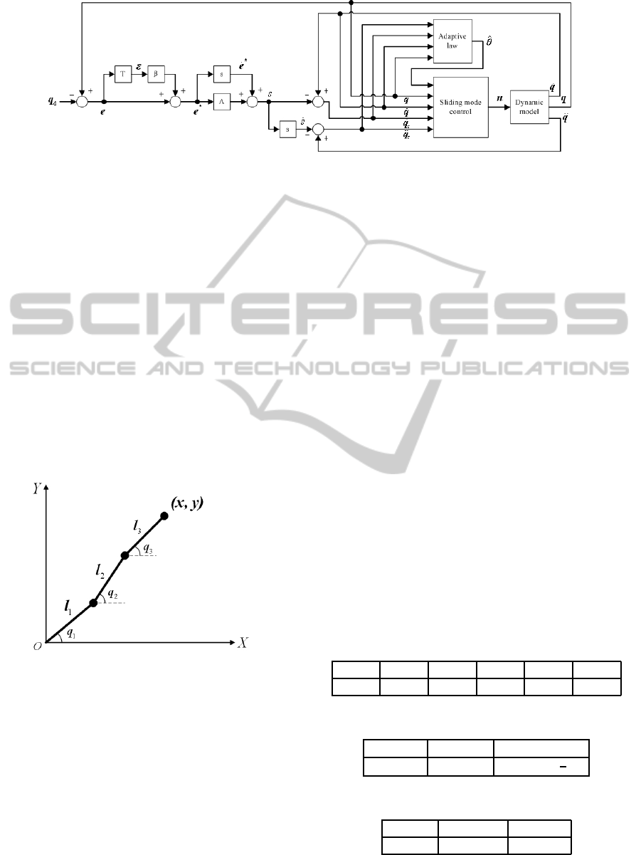
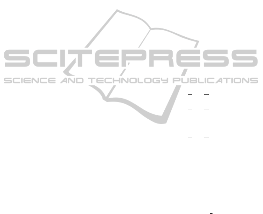
Figure 1: The Block diagram of the proposed controller.
robot manipulators. On one hand, the proposed con-
trol algorithm addresses the convergence of joint po-
sition tracking errors e
i
(t). On the other hand, it illus-
trates how these errors converge to zero, maintaining
synchronization errors ε
i
(t) → 0. And the proposed
controller can satisfy the transient performance of the
joint position tracking. The proposed control algo-
rithm can be depicted in Fig. 1.
4 SIMULATION
To validate effectiveness of the proposed approach,
simulations were performed on a 3-link planar robot
manipulator, as shown in Fig. 2, which dynamic
model is derived by methods in (Spong and Hutchin-
son, 2006).
Figure 2: A 3-link planer robot manipulator.
The dynamic parameter model of 3-link non-
linear planer robot manipulator in Eq. (1) is as follow:
M
11
M
12
M
13
M
21
M
22
M
23
M
31
M
32
M
33
¨q
1
¨q
2
¨q
3
+
C
11
C
12
C
13
C
21
C
22
C
23
C
31
C
32
C
33
˙q
1
˙q
2
˙q
3
+
g
1
g
2
g
3
+
d
1
(t)
d
2
(t)
d
3
(t)
= u
(22)
where the parameters in the matrices above can be
referred to the Eq. (23).
M
11
= m
1
l
2
1
+ (m
2
+ m
3
)l
2
1
+ i
1
,
M
12
= M
21
= (m
2
l
1
l
2
+ m
3
l
1
l
2
)cos(q
2
− q
1
),
M
13
= M
31
= m
3
l
1
l
3
cos(q
3
− q
1
),
M
22
= m
2
l
2
2
+ m
3
l
2
2
+ i
2
,
M
23
= M
32
= m
3
l
2
l
3
cos(q
3
− q
2
),
M
33
= m
3
l
2
3
+ i
3
,
C
11
= C
22
= C
33
= 0,
C
12
= − ˙q
2
(m
2
l
1
l
2
+ m
3
l
1
l
2
)sin(q
2
− q
1
),
C
13
= − ˙q
3
m
3
l
1
l
3
sin(q
3
− q
1
),
C
21
= ˙q
1
(m
2
l
1
l
2
+ m
3
l
1
l
2
)sin(q
3
− q
1
),
C
23
= − ˙q
3
m
3
l
2
l
3
sin(q
3
− q
2
),
C
31
= ˙q
1
m
3
l
1
l
3
sin(q
3
− q
1
),
C
32
= ˙q
2
m
3
l
2
l
3
sin(q
3
− q
2
),
g
1
= g[m
1
l
1
+ (m
2
+ m
3
)l
1
]cosq
1
,
g
2
= g(m
2
l
2
+ m
3
l
2
)cosq
2
,
g
3
= gm
3
l
3
cosq
3
.
(23)
In the simulation, the robotic manipulator param-
eter values are m
1
= 0.5kg, m
2
= 1.5kg, m
3
= 1.3kg,
l
1
= l
2
= l
3
= 1m, r
1
= r
2
= r
3
= 0.5m, where m
i
is
the link mass, l
i
is the link length and r
i
is the cen-
troid length. The moment of inertia are i
1
= 2kg · m
2
,
i
2
= 2kg · m
2
and i
3
= 2kg · m
2
.
Table 1: The initial conditions of the robot manipulator.
q
1
(0) q
2
(0) q
3
(0) ˙q
1
(0) ˙q
2
(0) ˙q
3
(0)
8 -9 1.5 8 -9 1.5
Table 2: The desired joint position.
q
d
1
(t) q
d
2
(t) q
d
3
(t)
sin(3πt) cos(3πt) sin(3πt +
1
3
π)
Table 3: The bounded disturbance.
d
1
(t) d
2
(t) d
3
(t)
5sin(t) 2.5cos(t) 5sin(2t)
The initial conditions and desired joint positions
of the robot manipulator were selected in Table 1 and
ICINCO2015-12thInternationalConferenceonInformaticsinControl,AutomationandRobotics
242
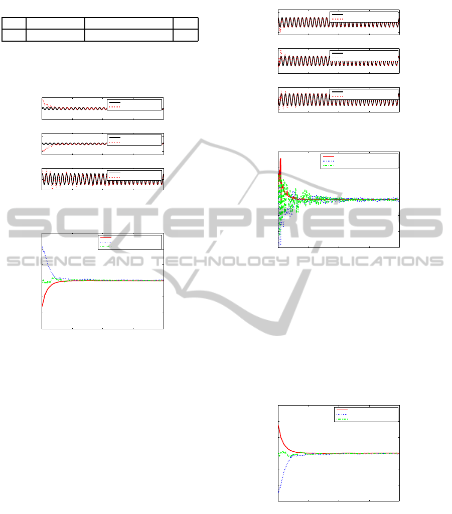
Table 4: The control gains.
β Λ K
r
α
0.1 diag[1, 1, 1] diag[300, 300, 300] 0.6
2. The bounded disturbance were set in Table 3. The
control gains in Eqs.(9), (10) and (11) were chosen in
Table 4.
0 5 10 15 20
−10
0
10
time/s
Angle/rad
Desired joint position 1
Joint position tracking 1
0 5 10 15 20
−10
0
10
time/s
Angle/rad
Desired joint position 2
Joint position tracking 2
0 5 10 15 20
−2
0
2
time/s
Angle/rad
Desired joint position 3
Joint position tracking 3
Figure 3: Joint position tracking response.
0 5 10 15 20
−15
−10
−5
0
5
10
15
time/s
Angle/rad
Joint position tracking error 1
Joint position tracking error 2
Joint position tracking error 3
Figure 4: Joint position tracking error output.
Figs. 3 and 4 illustrate the synchronized joint
position tracking response and error output of the
robotic manipulator with the proposed adaptive slid-
ing mode control (α 6= 0) under various disturbances.
The transient response and performance in joint posi-
tion tracking is better than the preview work in (Hu
and Liu, 2014), for comparison.
The synchronized joint position tracking errors
in Fig. 4 will converge to the neighbourhood in fi-
nite time (t = 3s), which reflects that the proposed
adaptive sliding mode control has a faster conver-
gence speed than the traditional sliding mode con-
troller. And it shows that the control gain Λ affects
the convergence speed in simulations. Else, the pro-
posed adaptive sliding mode control spends less time
to perform the simulations, which is caused by the
parameter α. The conclusion from Theorem 1 is not
only proved by the analysis, but also by the simula-
tions.
The synchronized joint position velocity tracking
response and errors of the robotic manipulator with
the proposed adaptive sliding mode control (α 6= 0)
under various disturbances are shown in Figs. 5 and
6. The proposed adaptive sliding control has a better
0 5 10 15 20
−20
0
20
time/s
Angle velocity/(rad/s)
Desired joint position velocity 1
Joint position velocity tracking 1
0 5 10 15 20
−20
0
20
time/s
Angle velocity/(rad/s)
Desired joint position velocity 2
Joint position velocity tracking 2
0 5 10 15 20
−20
0
20
time/s
Angle velocity/(rad/s)
Desired joint position velocity 3
Joint position velocity tracking 3
Figure 5: Joint position velocity tracking response.
0 5 10 15 20
−15
−10
−5
0
5
10
15
time/s
Angle/(rad/s)
Joint position velocity tracking error 1
Joint position velocity tracking error 2
Joint position velocity tracking error 3
Figure 6: Joint position velocity tracking error output.
synchronized joint position velocity tracking transient
response and performance than the results in (Hu and
Liu, 2014). It can be seen that the neighbourhood or
bound range is not only much smaller than the pre-
view results, but also is getting smaller.
Besides, from the simulations above, the pro-
posed adaptive sliding mode control does not require
the precise dynamic model of the robot manipulator,
which makes it very practical.
0 5 10 15 20
−15
−10
−5
0
5
10
15
time/s
Angle/rad
Coupled joint position error 1
Coupled joint position error 2
Coupled joint position error 3
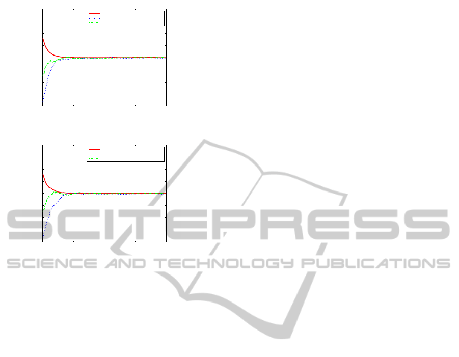
Figure 7: Coupled joint position error output.
Simulation results in Figs. 7, 8 and 9 display the
coupled joint position error and synchronized joint
position error (β 6= 0 and β = 0). These user-defined
joint position errors will converge to the bound range
in finite time. But the transient response and perfor-
mance of synchronized joint position errors output in
Figs. 8 and 9 is quite different, which is caused by the
control gain parameter β. From the simulations in Fig.
9, synchronized joint position error ε
3
(t) will con-
AnAdaptiveSlidingModeControllerforSynchronizedJointPositionTrackingControlofRobotManipulators
243
0 5 10 15 20
−20
−15
−10
−5
0
5
10
15
20
time/s
Angle/rad
Synchronization joint position error 1
Synchronization joint position error 2
Synchronization joint position error 3
Figure 8: Synchronized joint position error (β 6= 0).
0 5 10 15 20
−20
−15
−10
−5
0
5
10
15
20
time/s
Angle/rad
Synchronization joint position error 1
Synchronization joint position error 2
Synchronization joint position error 3
Figure 9: Synchronized joint position error (β = 0).
verge to the neighbourhood in advance. While, syn-
chronized joint position errors ε
1
(t), ε
2
(t) and ε
3
(t)
will converge simultaneously in Fig. 8.
5 CONCLUSIONS
We have proposed a novel adaptive sliding mode con-
troller for synchronized joint position tracking con-
trol of robotic manipulator. The proposed algorithm
does not require the precise dynamic model, and is
very practical than the traditional sliding mode con-
troller. On one hand, the proposed one addresses
a better convergence to zero of both joint position
tracking errors and joint position velocity tracking er-
rors. On the other hand, it ensures the transient re-
sponse and performance of synchronized joint posi-
tion tracking. And, the proposed controller maintain
the synchronized joint position errors will converge
to the neighbourhood simultaneously. Simulation re-
sults obtained from a 3-link non-linear planer robot
manipulator demonstrate the effectiveness of the ap-
proach under various disturbances.
ACKNOWLEDGEMENTS
The work here is supported by the National Sci-
ence and Technology Supporting Plan (Grant No.
2015BAF01B04), Collaborative Innovation Center
of High-End Manufacturing Equipment, the State
Key Basic Research Program of China (Grant No.
2011CB706903), the National Natural Science Foun-
dation of China (Grant No. 51175208), the Funda-
mental Research Funds for the Central Universities
(Grant Nos. 2013ZZGH001 and 2014CG006).
REFERENCES
Ge, M. and Guan, Z. H. (2012). Robust mode-free slid-
ing mode control of multi-fingered hand with position
synchronization in the task space. In Proceeding of the
5th International Conference on Intelligent Robotics
and Applications.
Guo, Y. Z. and Woo, P. Y. (2003). Adaptive fuzzy sliding
mode control for robotic manipulators. In Proceeding
of 42nd IEEE Conference on Decision and Control,
pages 149–159, Hawaii. IEEE.
Ho, H. F. and Wong, Y. K. (2007). Robust fuzzy track-
ing control for robotic manipulators. Simulation Mod-
elling Practice and Theory, 15(7):801–816.
Hu, Y. M. and Liu, J. (2014). Seam tracking control of weld-
ing robotic manipulators based on adaptive chattering-
free sliding-mode control technology. In Proceed-
ing of 11th International Conference of Informatics in
Control, Automation and Robotics. INSTICC.
Koren, Y. (1980). Cross-coupled biaxial computer con-
trols for manufacturing systems. ASME Journal
of Dynamic Systems, Measurement and Control,
102(4):265–272.
Liu, Y. C. and Chopra, N. (2012). Controlled synchroniza-
tion of heterogeneous robotic manipulators in the task
space. IEEE Transactions on Robotics, 28(1):268–
275.
Sage, H. G. and Mathelin, M. F. (1999). Robust control of
robot manipulators: a survey. International Journal of
control, 72(16):1498–1522.
Slotine, J. E. and Li, W. (1989). Composite adaptive control
of robot manipulators. Automatica, 25:509–519.
Slotine, J. E. and Li, W. P.(1987). On the adaptive control of
robot manipulators. International Journal of Robotics
Research, 6(3):49–59.
Slotine, J. E. and Li, W. P. (1991). Applied Nonlinear Con-
trol. Prentice Hall, Englewood Cliffs.
Spong, M. W. and Hutchinson, S. (2006). Robot Modeling
and Control. John Wiley & Sons, New York.
Sun, D. (2003). Position synchronization of multiple mo-
tion axes with adaptive coupling control. Automatica,
39:997–1005.
Sun, D. and Mills, J. K. (2002). Adaptive synchronized
control for coordination of two robot manipulators.
In Proceeding of IEEE International Conference on
Robotics and Automation, pages 976–981, Washing-
ton DC. IEEE.
Sun, D. and Shao, X. (2007). A model-free cross-coupled
control for position synchronization of multi-axis mo-
tions: theory and experiments. IEEE Transaction on
Control Systems Technology, 15(2):306–314.
ICINCO2015-12thInternationalConferenceonInformaticsinControl,AutomationandRobotics
244

Wang, X. and Zhang, J. (2015). Switched adaptive tracking
control of robot manipulators with fiction and chang-
ing loads. International Journal of Systems Science,
46(6):955–965.
Yang, Y. H. and Su, Y. X. (2008). Adaptive synchronized
control of robot manipulators. Journal of System Sim-
ulation, 20(1):117–119.
Zhao, D. and Li, C. X. (2011). Low-pass-filter-based posi-
tion synchronization sliding mode control for multiple
robotic manipulator systems. In Proceedings of the In-
stitution of Mechanical Engineers, pages 1136–1148.
AnAdaptiveSlidingModeControllerforSynchronizedJointPositionTrackingControlofRobotManipulators
245
