Global Surface Temperature Model using Coupled Sugeno Type Fuzzy

Inference Systems and Neural Network Optimization

Bernardo Bastien-Olvera

and Carlos Gay-Garcia

1,2

Climate Change Research Program, National University of Mexico, Mexico City, Mexico

Centre for Atmospheric Science, National University of Mexico, Mexico City, Mexico

Keywords:

Cimate Change, Global Temperature, Carbon Emissions, Fuzzy Inference Systems, Neural Networks.

Abstract:

In this research, a model that projects the mean global temperature as a function of anthropogenic carbon

emissions was generated with two fuzzy inference systems, sugeno type. We propose that the climatic system

is energetically balanced, and the albedo, solar constant and atmospheric transparency are all constants. Nev-

ertheless, we assume that the surface temperature varies when the CO

concentration changes and depends on

the system temperature itself. The second assertion states that any change in atmospheric CO

concentration

depends on anthropogenic carbon emissions and the system actual concentration. The fuzzy inference systems

were optimized using artiﬁcial neural networks that adjust the parameters according to a different data base

that the one that was used to create the initial system. So that, we assure to ﬁnd the hidden patterns and avoid

overﬁtting. The principal results of this work are the temperature projections under IPCC scenarios and the

discovering of the historical data hidden patterns.

1 INTRODUCTION

Climatic system is primarily driven by solar radiation

and its interaction with the atmospheric greenhouse

gases. In the most recent IPCC assessment report is

stated that is very likely that anthropogenic activity

increases global warming, so that, it is important to

generate efﬁcient models that project future climate,

based in possible emissions scenarios that will allow

the experts to plan mitigation and adaptation strate-

gies. A better description of a single component of the

system is given by simple models like an energy bal-

ance model (Budyko, 1969), in that sense we propose

in this work a model that projects the mean surface

global temperature, that assume that climatic system

is in a balance that would possibly be altered just by

the change in atmospheric CO

concentration. This

model had been constructed using fuzzy logic (Zadeh,

1965), which mathematical structure allows to repre-

sent in a very accurate way the fuzzy nature of the

problem in terms of the uncertainty of the involved

processes. We have created two coupled fuzzy infer-

ence systems (Zadeh, 1975), sugeno type (Takagi and

Sugeno, 1985), which causally relate input fuzzy sets

to linear regression equations in certain degree that

depends on the membership degree of the input vari-

able to the different fuzzy sets of the input universe.

The fuzzy inference systems of the model were

automatically constructed by MATLAB’s fuzzy logic

toolbox using a certain set of historical data, and then

we optimized the parameters using neural networks

(Jang et al., 1997) that worked with other data sets.

Finally, we obtained a model that ﬁts very well the

historical data and the temperature behaviour from the

past 50 years using historical emissions with a gener-

ated noise. The model is also used to project future

temperature based on the IPCC emissions scenarios.

This kind of models had been recently explored in

order to deal better with the complex interaction be-

tween physics of climate change and policy-makers

(Gay-Garcia and Sanchez-Meneses, 2015). While

models can be improved by the better understanding

of the climatic system, the emissions scenarios will be

always uncertain because they depend of the society’s

development and political decisions, that is the rea-

son why experts promote the implementation of mod-

els that are more tolerant to uncertainty (Gay-Garcia

et al., 2014).

2 MODEL PROPOSED

We have two basic statements in which this model

relies on. First, the planet is in energetic equilib-

519

Bastien-Olvera B. and Gay-Garcia C..

Global Surface Temperature Model using Coupled Sugeno Type Fuzzy Inference Systems and Neural Network Optimization.

DOI: 10.5220/0005524805190525

In Proceedings of the 5th International Conference on Simulation and Modeling Methodologies, Technologies and Applications (MSCCES-2015), pages

519-525

ISBN: 978-989-758-120-5

 2015 SCITEPRESS (Science and Technology Publications, Lda.)

rium, where the effective temperature, solar constant,

albedo and atmospheric transparency are all con-

stants, and, surface temperature (T ) only varies with

the change of atmospheric CO

concentration (Q) and

temperature rate of change is function of the temper-

ature itself (equation (2)). Secondly, we state that

any change in atmospheric CO

concentration is func-

tion of CO

emissions (E) and the concentration itself

(equation (1)).

= f (Q, E) (1)

= g





(2)

As we can see, equation (2) depends on the result

of equation (1). Since we will work with historical

data to obtain the behaviour of these equations, they

will transform into discrete equations:

∆Q

i+1

= g (Q

, E

) (3)

∆T

i+2

= f (∆Q

i+1

, T

i+1

) (4)

2.1 Fuzziﬁcation

We can fuzzify the equations (3) and (4) by giving

them a structure as follows:

∆Q

i+1

= p

+ q

, E

∈ A

(5)

∆T

i+2

= r

∆Q

i+1

+ s

i+1

∆Q

i+n

, T

i+1

∈ A

(6)

Where A

is the n − th fuzzy set of each universe

of variables (Temperature, Concentration and Emis-

sions). We deﬁned linguistically A

as the set of low

Temperature/Concentration/Emissions, A

: medium

and A

: high. When we give a pair of input variables

into equation (5), the system evaluates the member-

ship degree of the elements to the fuzzy set A

and

evaluates the equation using the parameters p

, q

then it does the same for the fuzzy sets A

and A

and the ﬁnal result will be the weighted sum of the

three last results. Then, the output of equation (5)

will be the input for equation (6) and the process de-

scribed above will be repeated in order to obtain the

ﬁnal output, the temperature.

3 METHODOLOGY

The membership functions of the fuzzy sets and the

parameters p, q, r, s were obtained analysing time-

series of historical data (described in the Appendix)

with MATLAB’s fuzzy logic tool ’genﬁs3’. Then we

optimized them using ’anﬁs’ the adaptive neuro-fuzzy

inference system tool that uses neural network the-

ory and works with the same data from which the

model was constructed, ﬁnally, we used a different

data set that control the optimization and prevents

over-ﬁtting. Guided by the training error we decided

to stop the optimization process whenever the error

stops decreasing (either the training error or the con-

trol error), we reach that point after 10 epochs for the

ﬁrst Fuzzy Inference System (FIS-1), while the sec-

ond Fuzzy Inference System (FIS-2) was trained 50

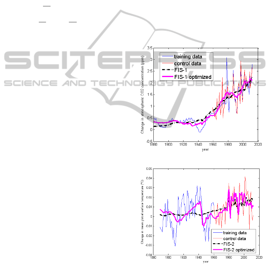
epochs. The results of the optimization can be seen

in the Figure 1 and 2, as it can be observed, the op-

timized FIS describe better the path from the original

data.

Figure 1: FIS-1 performance.

Figure 2: FIS-2 performance.

The ﬁnal part of the process was to generate a

simple script that uniﬁes both FIS as we can see in

the diagram of Figure 3. The ﬁrst two inputs are the

emissions and atmospheric concentration at year

SIMULTECH2015-5thInternationalConferenceonSimulationandModelingMethodologies,Technologiesand

Applications

520

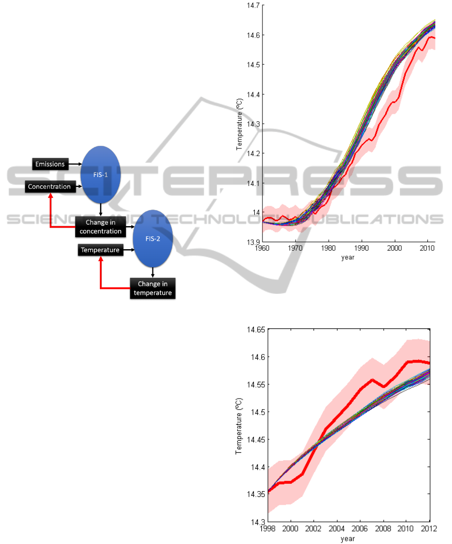
i which through the FIS-1, project the change in at-

mospheric CO

concentration at year i + 1. This last

variable works as input with the temperature at year

i + 1 in the FIS-2 that give us the change in tempera-

ture at year i +2. The next step is to add the change in

concentration of year i +1 to the concentration at year

i, and the temperature at year i + 2 is obtained adding

the change in temperature at year i + 2 to the temper-

ature at year i + 1; these steps are shown in red lines.

Finally, it only remains to give a value of the emis-

sions at year i + 2 so the second step of the model can

be complete and we can obtain the change in tempera-

ture at year i + 3 and so on. This means that when the

model completes one cycle, the only necessary input

is the emissions.

Figure 3: Model diagram.

3.1 Validation

We set the initial temperature and concentration val-

ues from 1959 and 1960 and we ran the model 50

times using the emissions from 1959 to 2010 adding

a noise which amplitude was equal to the uncertainty

of the data, every projection was different since the

added noise was randomly obtained every time. In

Figure 4 we note that 15 years after the ﬁrst step, some

projections start to be outside the error boundaries, so

we chose other 15 years to project the temperature,

and as we can see in Figure 5 those 15 years of pro-

jected temperature are inside of the error boundaries.

So we validated our model for the ﬁrst 15 years of

projection.

Furthermore, we created another model using only

historical data obtained before the year 2000. With

that second model we projected the temperature from

2000 to 2015 and compare it to the actual historical

data, that comparison serve as another method of val-

idation for our main model, it means that the method

actually works, since, as we can observe in Figure 6

almost every projected temperature is inside the

uncertainty band of the historical data.

Figure 4: 50 Projections of generated emissions with noise.

The red line is the historical data with its correspondient

uncertainty band (also in red), the other colored and thin-

ner lines are 50 projections made with historical emissions

adding random noise each time a projection is made.

Figure 5: 15 years of projections from 1998 to 2012. The

red line is the historical data with its correspondient uncer-

tainty band (also in red), the other colored and thinner lines

are 50 projections made with historical emissions adding

random noise each time a projection is made.

GlobalSurfaceTemperatureModelusingCoupledSugenoTypeFuzzyInferenceSystemsandNeuralNetwork

Optimization

521

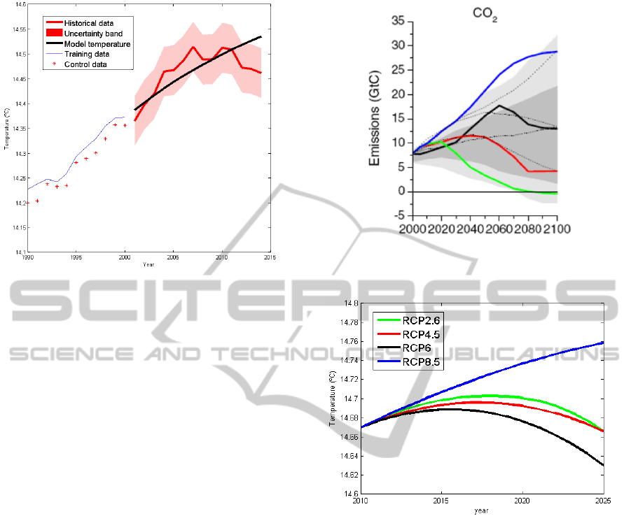
Figure 6: 15 years of projections from 2000 to 2015, using a

model created only with data collected befor the year 2000.

The red line is the historical data with its correspondient

uncertainty band (also in red), the black line is a projection

from 2000 to 2015 using the actual emissions. We also show

the training and control temperature data, the training data

goes back to 1880, the control data goes back to 1959.

4 PROJECTIONS

The principal and most controversial variable to

project in climate change is the greenhouse gases

emissions, so that it had been created some differ-

ent scenarios based on socio-economic assumptions

(Moss et al., 2007), these scenarios are standardized

so climate models can be compared between them.

IPCC’s AR5 proposed the representative concentra-

tion pathways (Figure 7) which we will use to project

future temperature with our model.

It is important to note the boundaries of the model.

The ﬁrst limitation is the 15 years that we deﬁned

as validated projections. Secondly, since the model

was made with historical data, the membership func-

tions of the fuzzy sets are just deﬁned for certain el-

ements of the variables universe. For the FIS-1, the

upper limit of the atmospheric CO

concentration in

which it works properly is around 440ppm and the

upper limit of the emissions is 15GtC. The FIS-2 up-

per limit for temperature is around 15 C. We made a

projection setting up the values at year 2010, accord-

ing to the validation, this projection will make sense

until 2025 (15 years of projection), which is the same

year when the RCP 8.5 reaches the upper limit of the

emissions in FIS-2. Figure 8 shows the 4 projections,

RCP8.5 is the only scenario where the temperature

is constantly increasing. We can note that, neverthe-

less the RCP2.6 temperature line is always above the

Figure 7: Emissions from the Representative Concentration

Pathways. (Van Vuuren et al., 2011).

Figure 8: Fuzzy model projections based on RCPs scenar-

ios.

temperature projected under RCP4.5, at the end of the

projections the rate of decrease is greater in the more

optimistic scenario, RCP2.6. It is also remarkable that

the lowest temperature projection is the one made un-

der the RCP6 scenario, which is not very straightfor-

ward to think intuitively, the hidden patterns, in the

next section, could help to discover why this happens.

5 DISCUSSION

The parameters of the model were obtained analysing

historical data and optimizing them using neural net-

work theory, which allow us to ﬁnd the hidden pat-

terns that relied on the data. The membership func-

tions were adjusted as well as the linear equation that

implies every fuzzy set.

The ﬁnal optimized parameters for the FIS-1 in-

ference rules are:

SIMULTECH2015-5thInternationalConferenceonSimulationandModelingMethodologies,Technologiesand

Applications

522

• If Emissions and Concentration are low:

∆C = 0.333Emissions − 0.025Concentration +

7.225

• If Emissions and Concentration are medium:

∆C = 0.563Emissions − 0.004Concentration −

0.513

• If Emissions and Concentration are high:

∆C = −0.417Emissions + 0.055Concentration −

14.972

As we can see in the equations above, when the

emissions and concentration parameters go from low

to high, the concentration becomes a factor of incre-

ment of itself, this talks about a positive feedback, and

it could be related to some biotic cycles such as ocean

acidiﬁcation and its interaction with corals. Another

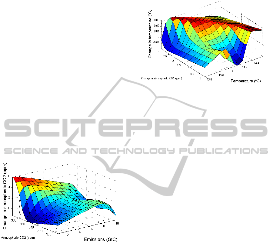
way to view the rules and parameters is with the rules

surface, as shown in Figure 9 where we can observe

that the change in atmospheric CO

increases with

the increment of emissions as long as atmospheric

concentration is low. The increment decays with

the emissions when the atmospheric concentration is

high.

Figure 9: Rules surface of FIS-1.

The inference rules of the FIS-2 are:

• If Temperature and ∆C are low:

∆T = 0.066T − 0.005∆C − 0.9

• If Temperature and ∆C are medium:

∆T = −0.006T + 0.022∆C + 0.072

• If Temperature and ∆C are high:

∆T = −0.035T − 0.008∆C + 0.542

By studying the rules, we can say that the temper-

ature have a negative feedback, which can represent

that some processes, that are cooling down the sys-

tem, are triggered by high temperatures. The third

rule by itself is counter-intuitive, so we should see

the big picture: graphically displayed in Figure 10,

it is shown that the surface describing the change in

temperature is complex. If we do a transect with con-

stant change in atmospheric CO

concentration it can

Figure 10: Rules surface of FIS-2.

easily be observed that the change in temperature de-

scribes a cyclic variation, which amplitude increase

with greater temperatures and greater changes in at-

mospheric CO

. This pattern could describe that the

resilience of the system decays when the forcing in-

creases.

6 CONCLUSIONS

In order to face climate change, we should have

in mind the complexity of the system and have a

clear idea of the factors that play a role in this un-

precedented challenge. There had been developed a

great variety of climatic models and from them socio-

economic scenarios are generated and global politi-

cal decisions are taken. The greatest contribution of

this work, relies on the methodology of a fuzzy cli-

mate modelling that will allow to unify the differ-

ent faces of climate change, in which questions as:

’How does medium changes in temperature would af-

fect economic development in certain region?’ or

’What actions need to be taken in order to reduce

emissions into a low level?’, will be answered in

single-simulation processes;that way, policy-makers

will have a real efﬁcient tool to make the best possible

decision. The presented model is the initial phase of

a ground-breaking climate change modelling.

REFERENCES

Boden, T. A., Marland, G., and Andres, R. J. (2013).

Global, regional, and national fossil-fuel co2 emis-

sions.

Budyko, M. I. (1969). The effect of solar radiation varia-

tions on the climate of the earth. Tellus XXI, 5:611–

619.

Dlugokencky, E. and Tans, P. (2014). Trends in atmospheric

carbon dioxide. www.esrl.noaa.gov/gmd/ccgg/trends.

GlobalSurfaceTemperatureModelusingCoupledSugenoTypeFuzzyInferenceSystemsandNeuralNetwork

Optimization

523

Etheridge, D. M., Steele, L. P., Langenfelds, R. L., Francey,

R. J., Barnola, J. M., and Morgan, V. I. (1998). His-

torical co2 records from the law dome de08, de08-2,

and dss ice cores. Cdiac.ornl.gov.

Gay-Garcia, C. and Sanchez-Meneses, O. (2015). Fuzzy

climate scenarios for temperature indicate that things

could be worse than previously thought. Simulation

and Modeling Methodologies, Technologies and Ap-

plications, Advances in Intelligent Systems and Com-

puting.

Gay-Garcia, C., Sanchez-Meneses, O., Martinez-Lopez, B.,

Nebot, A., and Estrada, F. (2014). Fuzzy models: Eas-

ier to undestand and an easier way to handle uncertain-

ties in climate change research. Simulation and Mod-

eling Methodologies, Technologies and aplications,

Advances in intelligent System Computing.

Houghton, R. A., van der Werf, G. R., Hanses, R. S.,

House, M. C., Le Quere, C., Pongratz, J., and N., R.

(2012). Carbon emissions from land use and land-

cover change. Biogeosciences, 9:5125 – 5142.

Jang, J.-S. R., Sun, C.-T., and Mizutani, E. (1997). Neuro-

fuzzy and soft computing. Prentice Hall, Englewood

Cliffs, N.J.

Moss, R., Babiker, M., Brinkman, S., Calvo, E., Carter, T.,

Edmonds, J., Elgizouli, I., Emori, S., Erda, L., Hib-

bard, K., Roger, J., Kainuma, M., Kelleher, J., Lamar-

que, J. F., Manning, M., Matthews, B., Meehl, J.,

Meyer, L., Mitchell, J., Nakicenovik, N., O’Neill, B.,

Pichs, R., Riahi, K., Rose, S., Runc, P., Stouffer, R.,

van Vuuren, D., Weyant, J., Wilbanks, T., van Yper-

sele, J. P., and Zurek, M. (2007). Towards new scenar-

ios for analysis of emissions, climate change, impacts,

and response strategies. IPCC Expert meeting report.

NASA (2014). Giss surface temperature analysis (gistemp).

giss.nasa.gov.

Takagi, T. and Sugeno, M. (1985). Fuzzy identiﬁcation of

system and its application to modeling and control.

IEEE, SMC, 15:199–249.

Tans, P. and Keeling, R. (2014). Noaa/esrl. www.esrl.

noaa.gov/gmd/ccgg/trends.

Van Vuuren, D. P., Stehfest, E., Den Elzen, M. G. J., Deet-

man, S., A., H., Isaac, M., K., K. G., T., K., Mendoza-

Beltran, A., and Oostenrijk, R. (2011). Exploring the

possibility to keep global mean temperature change

below 2c. Climatic Change.

Zadeh, L. A. (1965). Fuzzy sets. Information and control,

8:338–353.

Zadeh, L. A. (1975). The concept of a linguistic variable

and its application to approximate reasoning. Inf. Sci,

8:199–249.

APPENDIX

Here we present the data used in the construction and

optimization of the model, also it is shown the data

that served as control. See Table 1

SIMULTECH2015-5thInternationalConferenceonSimulationandModelingMethodologies,Technologiesand

Applications

524

Table 1: Historical Data.

Variable Description Source

Data for Carbon Carbon emissions estimation (Boden et al., 2013)

model emissions by fossil fuels

construction (1880 - 2012).

and Carbon emissions estimation (Houghton et al., 2012)

optimization by land-use change

(1880 - 2012).

Atmospheric CO

Atmospheric carbon estimation (Etheridge et al., 1998)

through ice nuclei

(1880 - 1978).

Atmospheric carbon (Dlugokencky and Tans, 2014)

grow estimation (1980 - 2013).

Global temperature Mean global surface (NASA, 2014)

temperature estimation (1980 - 2013).

Data for Carbon Carbon emissionsobservations (Boden et al., 2013)

controlling emissions by fossil fuels

the optimization (1959 - 2013).

Carbon emissions observations (Houghton et al., 2012)

by land-use change

(1959 - 2012).

Atmospheric CO

atmospheric concentration (Tans and Keeling, 2014)

observations (1959 - 2013)

Global temperature Mean global surface (NASA, 2014)

temperature estimation (1959 - 2013)

GlobalSurfaceTemperatureModelusingCoupledSugenoTypeFuzzyInferenceSystemsandNeuralNetwork

Optimization

525