
Design, Analysis and Control of a Semi-active Magnetic Bearing System
for Rotating Machine Applications
T.-J. Yeh
Department of Power Mechanical Engineering, National Tsing-Hua University, Hsinchu, Taiwan, R.O.C.
Keywords:
Magnetic Bearing, Permanent Magnet, LTR Control.
Abstract:
In this paper, a semi-active magnetic bearing system which incorporates both the active and passive magnetic
bearings is proposed for rotating machine applications. Particularly, the design, analysis, and control issues of
the semi-active system are investigated by using an axial fan as the platform. In the proposed system, while
the rotor is levitated axially by the active bearing, its radial and tilting stabilities are guaranteed by the passive
bearings. By carefully designing the radial and tilting stiffnesses of the passive bearings and the controller
of the active bearing, the system can be successfully operated to the rated speed of 4000rpm. Because the
semi-active magnetic system is frictionless and consumes insignificant power in levitation, its total power
consumption is 14.7% less than the conventional fan in which mechanical ball bearings are used.
1 INTRODUCTION
The use of magnetic bearings in industrial applica-
tions has attracted increasing attention in recent years.
The major advantage offered by magnetic bearings is
that there is no physical contact between the bearing
and the levitated object, so friction is eliminated and
lubrication is not needed. In general, magnetic bear-
ings can be classified into two types: the active type
and the passive type. Active magnetic bearings are
made of electromagnets whose coil currents are con-
trolled based on the sensor measurements(T.-J. Yeh
and Wu, 2001)(Yeh et al., 2001). Active magnetic
bearings allow the system designers to flexibly ad-
just the bearing stiffness and damping, and inject ap-
propriate signals to cancel the undesired vibrations.
Nevertheless, due to the necessary control hardware
including sensors, control electronics/digital signal
processor, and power amplifiers, the use of active
magnetic bearings substantially increases system cost
and complexity. On the other hand, passive mag-
netic bearings are simply made of permanent mag-
nets and rely on either the attractive or repulsive mag-
netic force to achievelevitation (J. Delamare and Yon-
net, 1995)(H. Okuda and Ito, 1984)(Yonnet, 1981).
Passive magnetic bearings do not require any control
hardware as the active bearings do, so they are inex-
pensive and structurally simple. However, by Earn-
shaw’s theorem, total stability is not possible for sys-
tems containing only passive magnetic bearings. In
these systems, the object to be levitated always has
to be constrained mechanically in certain degrees of
freedom. As a result, physical contact is established
and frictional loss is induced.
Considering the pros and cons in magnetic bear-
ings, if one wants to keep the system complexity to
minimum and yet achieve total levitation, the most
economical solution will be a system combining the
favorable features from both types of the bearings,
or so-called the semi-active magnetic bearing system.
Semi-active systems have been reported by several re-
searchers. For example, in (J. Delamare and Rulli,
1994) an angularly stable radial bearing is incorpo-
rated with an active magnetic bearing in the axial di-
rection to levitate a rotor. However, due to the low
stiffness in the passive bearing, total levitation is not
possible for the whole range of speed that the rotor
has to start its rotation with ball bearings until the first
critical speed of 750rpm is passed. In (J.F. Antaki
and Groom, 2000)(J.F. Antaki and Groom, 2001), the
authors devised a magnetically levitated blood pump
as the artificial heart. In this system, the rotor is sus-
pended by two permanent magnet radial bearings and
an active magnetic thrust bearing which is actuated
by two voice coils. With the help of the blood as
the damping source, the system is capable of spin-
ning between 4000rpm and 8000rpm. In this paper,
the development of a semi-active magnetic bearing
system for rotating machine applications is demon-
strated by using a commercially available 127mm ×
503
Yeh T..
Design, Analysis and Control of a Semi-active Magnetic Bearing System for Rotating Machine Applications.
DOI: 10.5220/0005528205030510
In Proceedings of the 12th International Conference on Informatics in Control, Automation and Robotics (ICINCO-2015), pages 503-510
ISBN: 978-989-758-122-9
Copyright
c
2015 SCITEPRESS (Science and Technology Publications, Lda.)
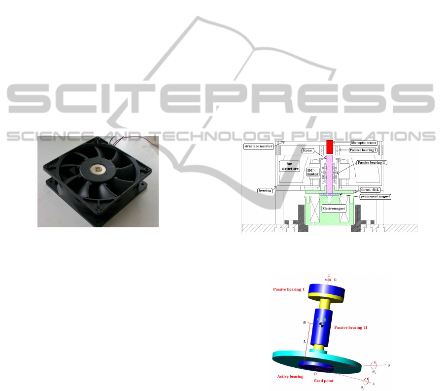
127mm ×38mm axial fan as the platform. The axial
fan, whose photograph is shown in Figure 1, is driven
by a brushless DC motor and uses axial air flow to
provide cooling for computer peripherals. Given the
limited space for mounting the magnetic bearings, the
requirement to spin to the rated speed of 4000rpm
without using any mechanical bearings, as well as
lack of fluid damping because the fan is operated in
the air, the development requires systematic proce-
dures in design, analysis, and control. The rest of
the paper is organized as follows: System configura-
tion and dynamic analysis of the semi-activemagnetic
bearing system are introduced in section 2. Section
3 discusses how the passive bearings are designed to
achieve the desired radial and tilting stiffnesses. In
section 4, the physical model of the active magnetic
bearing is first presented. Then system identifica-
tion and controller design are performed to stabilize
the bearing dynamics. Section 5 presents experimen-
tal verifications of the system performance. Finally,
conclusions are given in section 6.
Figure 1: Photo of the axial fan.
2 SYSTEM CONFIGURATION
AND DYNAMIC ANALYSIS
Figure 2 shows the schematic of the semi-active mag-
netic bearing system. There are one active magnetic
bearing and two passive magnetic bearings. The
active bearing consists of an annular electromagnet
and a thrust disk which contains a circular permanent
magnet with the same diameter as the inner pole face
of the electromagnet. This active bearing is used to
provide frictionless support to the rotor in the axial
direction. Since feedback is always needed for the ac-
tive bearing, a fiber-optic sensor, which measures ro-
tor’s axial position, is mounted on a structural mem-
ber whose both ends are in turn attached rigidly to the
top of the fan housing.
Passive bearing I is composed of two permanent
magnet rings with one on the top of the rotor and
the other attached to the same structural member on
which the senor is mounted. The two magnets are
polarized axially and are aligned with the rotor’s axis.
Because the magnets are placed in attractive manner,
an upward magnetic force is applied to the rotor. Pas-
sive bearing II consists of two concentric stacks of
permanent magnet rings respectively attached to the
rotor and the housing. The permanent magnet rings
are polarized axially and are stacked in a repelling
manner for squeezing more magnetic fluxes towards
the air gap between the stacks. The polarities of
the two stacks are arranged so that they repel against
each other. Moreover, because the magnetic poles of
the outer stack are not aligned with those of the in-
ner stack, passive bearing II applies an downard force
to the rotor. These two sets of passive bearings to-
gether serve two purposes. One is to provide tilting
and radial stiffnesses so that when the rotor tilts or
translates radially, a restoring torque or force can be
produced. The other is to provide a suitable upward
axial bias force for the active bearing to counteract.
Such a counteraction allows the active bearing, which
generates downward force only, to have full control of
rotor’s axial motion so as to generate axial stiffness.
Figure 2: Configuration of the semi-active magnetic bearing
system.
Figure 3: Definitions of variables for dynamic analysis.
The dynamic analysis follows the definitions of
variablesin Figure 3. For simplification, it is assumed
that the controller of the active magnetic bearing ren-
ders the rotor with high axial stiffness that the center
point of the thrust disk, or the point O in Figure 3, can
be treated as a fixed point in the free space. By do-
ing so, the rotor becomes an axially symmetric body
spinning about a fixed point. The rotor dynamics is
ICINCO2015-12thInternationalConferenceonInformaticsinControl,AutomationandRobotics
504
thus given by:
m
..
x+ k
r
x = meΩ
2
sinΩt (1)
m
..
y+ k
r
y = meΩ
2
cosΩt (2)
I
t
¨
θ
x
+ ΩI
a
˙
θ
y
+ (k
θ
−mgL)θ
x
= meΩ
2
LsinΩt(3)
I
t
¨
θ
y
−ΩI
a
˙
θ
y
+ (k
θ
−mgL)θ
y
= meΩ
2
LcosΩt(4)
where m is the mass of the rotor, I
t
is the trans-
verse moment of inertia about the fixed point, I
a
is
the axial moment of inertia, Ω is the rotor speed, x, y
and θ
x
, θ
y
are respectively the rotor’s radial displace-
ments and tilting angles, k
r
and k
θ
are the radial and
the tilting stiffnesses provided by the magnetic bear-
ings, L is the distance from rotor’s center of gravity
to the fixed point O, and e is the rotor unbalance. It
should be noted that while the first two equations are
from the translational dynamics, the last two are due
to the gyroscopic effect. Moreover, the right side
of the equations are caused by the unbalance forces
(torques) which are proportionalto meΩ
2
and are syn-
chronized with Ω.
By considering the resonance in the rotor dynam-
ics, one can compute the minimum bearing stiffnesses
needed for the rotor to successfully spin to the rated
speed of 4000rpm. Taking the the radial stiffness k
r
for example, in order to avoid resonance during accel-
eration of the rotor, it is desired to place the resonant
frequency above the rated speed. For m = 0.2kg and
the given rated speed, it can be shown from (1) or (2)
that k
r
has to be larger than 35,092
N
m
. The rotor in
consideration has a mass unbalance specification of
85µm. If keeping the amplitude of vibration within
0.25mm(which equals half of the bearing gap) at the
rated speed is desired, then the lower bound for k
r
is
raised to 47, 000
N
m
. To determine the tilting stiffness,
by taking Laplace transform on (3) and (4), it can be
found that if k
θ
> mgL, the rotor is stable with two
resonant frequencies:
ω
2
n1,n2
=
1
2I
2
t
2I
t
(k
θ
−mgL)+ Ω
2
I
2
a
±
p
Ω
4
I
4
a
+ 4I
t
(k
θ
−mgL)Ω
2
I
2
a
o
(5)
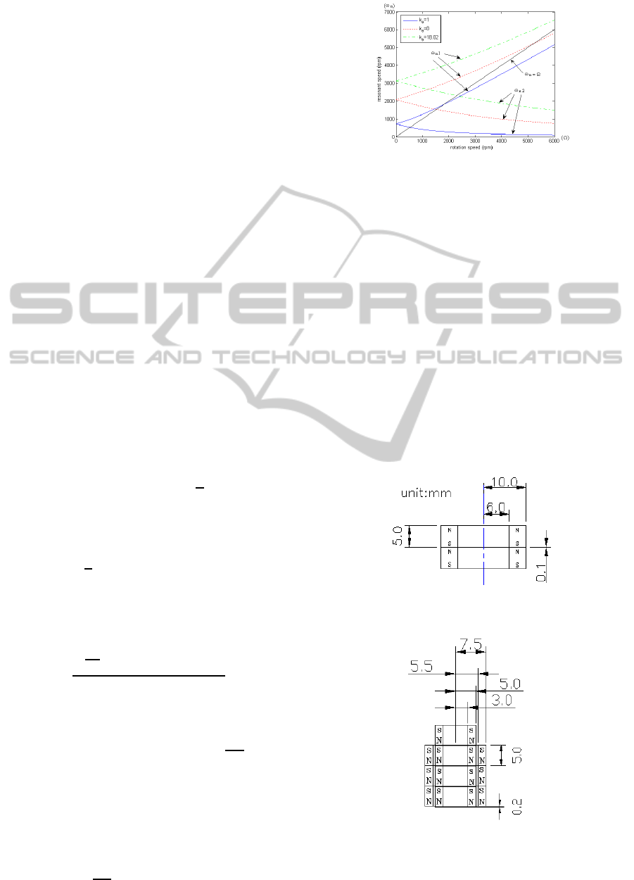
Figure 4 shows how ω
n1
, ω
n2
(in the unit of rpm)
vary with for I
a
= 1.4×10
−4
kg·m
2
, I
t
= 3×10
−4
kg·
m
2
, L = 0.022m, and k
θ
= 1, 8, 18.02
N·m
rad
. Ap-
parently, while ω
n1
increases with Ω, ω
n2
decreases
with Ω. When either one of the resonant frequencies
equals the rotation speed, resonance occurs. Ideally,
to avoid the resonance as Ω varies from zero rpm to
the rated speed, the two resonant curves should not
intersect with the ω
n
= Ω line in Figure 4. It can be
computed that to achieve such a condition k
θ
has to
be greater than 55
N·m
rad
.
Figure 4: Resonant speed v.s. rotation speed for different.
3 DESIGN AND ANALYSIS OF
PASSIVE MAGNETIC
BEARINGS
Although the lower bounds for the radial and tilting
stiffnesses can be computed via the dynamic analy-
sis, it is still desired to make the stiffnesses as high as
possible for minimizing rotor’s vibration during spin-
ning. However, as implied by Earnshaw’s theorem,
the stable radial and tilting stiffnesses simultaneously
induce instability in the axial direction and indeed the
instability increases with the stable stiffnesses. In siz-
ing the passive bearings, other than pursuing high ra-
dial and tilting stiffness, the axial instability also has
to be kept low so that the active bearing is able to
compensate.
Figure 5: Schematics of Passive Bearing I.
Figure 6: Schematics of Passive bearing II.
In this research, a finite-element package(ans, )
is employed to analyze the relevant bearing proper-
Design,AnalysisandControlofaSemi-activeMagneticBearingSystemforRotatingMachineApplications
505

ties including stiffnesses and instabilities so that a
better compromise among the design parameters can
be achieved. The magnetic material used here is
NdFeB with the remanence magnetic flux density of
1.23Telsa. The schematics of two passive bearings
obtained after several design iterations are shown re-
spectively in Figure 5 and Figure 6. Particularly, in
passive bearing II, while the outer stack consists of
three magnetic rings, the inner stack consists of four
magnetic rings, and the magnetic poles of the outer
stack are dislocated from those of the inner stack by
0.2mm in the downward manner.
Table 1: Properties of the Passive Bearings.
Passive
Bearing I
Passive
Bearing II
Radial Stiffness 8,000
N
m
38,000
N
m
Tilting Stiffness 16.62
N·m
rad
1.4
N·m
rad
Axial Instability 26,300
N
m
74,400
N
m
Axial bias force 49.44N −21.2N
The radial stiffness, tilting stiffness, axial stabil-
ity and the upward force respectively provided by the
two passive bearings are listed in Table 1. According
to this table, the tilting stiffness is mainly contributed
by passive bearing I and the radial stiffness is mainly
contributed by passive bearing II. In order to keep
the axial instability to minimum, we deliberately limit
the radial stiffness of passive bearing II, which is the
main source of axial instability, to 38, 000
N
m
by hav-
ing unequal numbers of magnetic rings for the inner
and outer stack
1
. The total radial stiffness in this case
is only 46,000
N
m
, which is still 1, 000
N
m
less than the
lower bound computed in previous section. As will
be shown later, the additional radial stiffness needed
will be provided by the active bearing. From the ta-
ble it can also be found that the total tilting stiffness is
only 18.02
N·m
rad
, which means that the rotor will expe-
rience a resonance at 2,200rpm. Due to the limited
space for placing the magnets and the unavailability
of magnets of extreme strength, it is difficultto further
increase the tilting stiffness to avoid the resonance.
In the following investigation, this tilting stiffness is
adopted, so as the rotor accelerates towards the rated
speed, it will experience resonance shortly. Since the
unbalance force is small at low speeds, as long as the
1
The finite element simulations indicate that if the inner and
outer stacks of passive bearing II both have three rings,
then the radial stiffness is only 33.450
N
m
. If the number
of rings for both stacks are increased to four, the radial
stiffness becomes 44,510
N
m
but the axial instability also
becomes excessive. As a comprimise, unequal number of
rings are adopted respectively for the outer (3) and inner
(4) stack.
rotor accelerates fast enough, it will not collide with
the stator and such resonance will be acceptable. Fi-
nally, the dislocation between the concentric stacks
of bearing II induces a downward axial bias force of
21.2N to the rotor. This downward force is used to
cancel part of the upward force from bearing I. By
doing so, the total upward force that the active bearing
has to counteract is not excessive and thus its power
consumption at steady state is reduced.
4 MODELING, IDENTIFICATION,
AND CONTROL OF THE
ACTIVE MAGNETIC BEARING
In the active magnetic bearing, if the magnetic flux
leakage, fringing flux, and the magnetic reluctance in
the iron core are ignored, one can derive the following
magnetic force equation:
F
m
=
−A
2
[µ
0
Ni+ B
r
l/µ
r
]
2
2µ
0
(z+ l/µ
r
)
2
(1+ A
2
/A
1
)
(6)
where F
m
is the downward magnetic force generated,
µ
0
is the air permeability, µ
r
and B
r
are respectively
the relative permeability and the remanence magnetic
flux density of the permanent magnet, z is the air gap,
µ
0
is the air permeability, i is the coil current, N is
the number of coil turns, l is the thickness of the per-
manent magnet, A
1
and A
2
are respectively the areas
of the inner(circular) and outer(annular) pole faces.
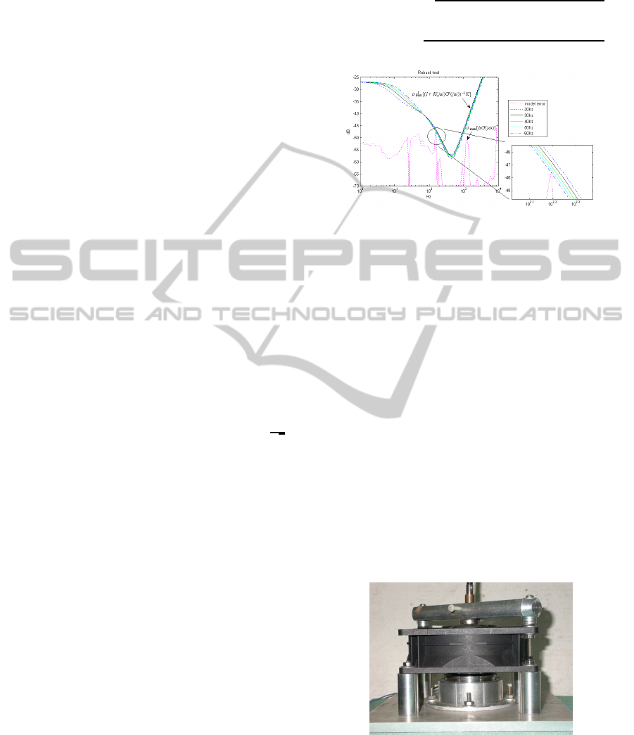
Table 2 lists the numerical values of the relevant pa-
rameters for the active magnetic bearing. Comparing
the magnetic force computed by (6) with the finite-
element simulations, it can be found that the theo-
retical equation tends to overestimate the magnetic
force because it ignores the magnetic flux leakage and
fringing flux associated with the permanent magnet.
To make a more accurate force prediction, one can in-
troduce a correction factor η in which ηl replaces l in
(6) as the equivalent thickness of the permanent mag-
net. By choosing η to be 0.946, Figure 7 shows that
the theoretical equation matches the finite element re-
sults better with maximum error less than 3%.
4.1 Linear Model and Identification
To facilitate the subsequent linear control design, the
nonlinear force equation (6) with the correction factor
is linearized around i = 0, and z = z
0
, where z
0
is the
nominal air gap. The linearization results in
F
m
≈ −k
i
δi+ k
s
δz−F
b
(7)
ICINCO2015-12thInternationalConferenceonInformaticsinControl,AutomationandRobotics
506
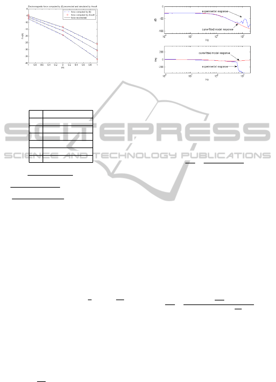
Figure 7: Comparisions of the force equations with the
finite-element results.
Table 2: The numerical values of the relevent parameters
for the active magnetic bearing.
A
1
3.14×10
−4
(m
2
)
A
2
7.06×10
−4
(m
2
)
µ
0
4π ×10
−7
N 300 (turn)
B
r
0.55 (T)
l 2×10
−3
(m)
µ
r
1.06
where k
i
=
A
2
NB
r
ηl/µ
r
(z
o
+ηl/µ
r
)
2
(1+A
2
/A
1
)
is the current gain,
k
s
=
A
2
[B
r
ηl/µ
r
]
2
µ
0
(1+A
2
/A
1
)(z
o
+ηl/µ
r
)
3
is the unstable stiffness,
F
b
=
A
2
(B
r
ηl/µ
r
)
2
2µ
0
(z
0
+ηl/µ
r
)
2
(1+A
2
/A
1
)
is the downward bias
force provided by the permanent magnet, δi and δz
denote the perturbations in current and axial displace-
ment respectively. If z
0
is selected to be 0.2mm, then
F
b
≈ 21.385N. This bias force, when combined with
the rotor’s weight, cancel most of the upward force
from the passive bearings. Therefore, if the ac-
tive bearing is stabilized at this nominal air gap, the
steady-state power required for levitation is insignifi-
cant.
It should be noted that although the active bearing
is open-loop unstable in the axial direction, it is sta-
ble in the radial and tilting directions. Finite element
simulations reveal that the associated radial and tilt-
ing stiffnesses are respectively 1,000
N
m
and 0.01
N·m
rad
.
Although the tilting stiffness is minuscule compared
to those offered by the passive bearings, as mentioned
in the previous section that such a radial stiffness is
just enough to limit rotor’s amplitude of vibration
to within half of the airgap as the rotor accelerates
towards the rated speed. Assume that the passive
bearings’ downward force balances with the rotor’s
weight and permanent’s bias force, the linearized dy-
namic equation for the axial motion can be derive as
m
d
2
z
dt
= (k
s
+ k
p
)z−k
i
i (8)
Figure 8: Frequency responses of the active magnetic bear-
ing.
where k
p
is the total axial instability contributed by
the two passive bearings. Notice that in this equa-
tion the perturbation symbol δ associated with i and z
has been removed for simplicity. By substituting the
respective numerical values into (8) and then taking
Laplace transform, the system transfer function G(s)
can be computed as
G(s) =
z(s)
i(s)
=
−11.9
0.2s
2
−114,000
(9)
System identification is performed on the active
bearing to experimentally identify the transfer func-
tion. The identification is based on frequency re-
sponse tests. Because the system is open-loop unsta-
ble, the identification is performed in closed loop by
using a PID controller to stabilize the system. Dur-
ing the identification test, a sinusoidal signal, whose
frequency ranges from 10Hz to 10kHz, is injected as
a disturbance and the frequency response is obtained
by comparing the amplitudes and phases of the coil
current and the rotor position.
In Figure 8, the experimental frequency response
is shown. This frequency response is also curve-
fitted by a transfer function which retains the form
of the theoretical input-output behavior in (9) except
that one extra pole and zero are added. The transfer
function, given by
G(s) =
z(s)
i(s)
=
−10(
s
5027
+ 1)
(0.21s
2
−100,000)(
s
942
+ 1)
(10)
is also plotted in Figure 8. The second order part of
this transfer function, which has phase of zero for all
frequencies, only differs slightly from the theoretical
model, and the extra pole and zero added are used to
account for the additional phase lag for ω > 10Hz. It
should be noted that the experimental frequency re-
sponse matches the curve-fitted transfer function ex-
cept for the first structural frequency at about 200Hz
and other structural modes occurring at ω > 500Hz.
Therefore, the transfer function in (10) will be used
Design,AnalysisandControlofaSemi-activeMagneticBearingSystemforRotatingMachineApplications
507
as the nominal model and its discrepancy from the ex-
perimental frequency response will be treated as the
modeling error in the following controller design.
4.2 LTR Controller Design
The PID controller designed for identification, al-
though is simple and stabilizing, has limited perfor-
mance due to its restricted control structure and trial-
and-error nature. Experimentally, the axial stiff-
ness provided by the PID controller is too compli-
ant for the rotor to spin. In this section, we use the
loop-transfer-recovery(LTR) design to systematically
devise a high-performance controller to increase the
stiffness of the active bearing.
In order for the control system to be stiff enough
to reject disturbances at low frequencies, an integrator
is augmented to G(s) and then the LTR design is con-
ducted on the state-space representation of the aug-
mented system. LTR is a linear quadratic Gaussian
(LQG) optimal control based method. The design
procedure requires one to solve two algebraic Riccati
equations: one corresponds to the Linear Quadratic
Regulator problem, and the other to the Kalman Fil-
ter problem. As shown in (Athans, 1986), by im-
plementing the cheap control LQR problem in LQG,
the system’s loop transfer function can be recovered
to a Kalman filter loop transfer function which mim-
ics a pure integrator with a bandwidth equal to
1
√
µ
,
where µ is a fictitious output noise intensity. This in-
dicates that the LTR design allows one to designate
the closed-loop system bandwidth by the choice of µ.
Ideally the closed-loop bandwidth should be set as
high as possible so that the system can achieve better
disturbance rejection. However, the higher the band-
width, the less likely the control system can maintain
the robust stability against the modeling error. To se-
lect the appropriate bandwidth, we employ the small-
gain result (K. Zhou and Glover, 1996) which, when
applied to the current case, states that given a nominal
model G with additive modeling error ∆G, a stabiliz-
ing controller K can provide robust stability if
|∆G( jω)| <
(1+ K(jω)G( jω))
−1
K(jω)
. (11)
Figure 9 plots
(1+ K( jω)G( jω))
−1
K(jω)
corre-
sponding to several different designated bandwidths
as well as |∆G( jω)|which denotes the modeling error
between G and the experimental frequency response
in Figure 8. It is clear that when ω
b
is raised to 60Hz,
the two functions in (11) intersect with each other at
the first structural frequency. Thus in the final LTR
design ω
b
= 50Hz is adopted and the controller is
given by
K
LQG
(s) = −
8.23×10
9
s
3
+ 1.358×10
13
s
2
s(s
4
+ 9224s
3
+ 4.157×10
7
s
2
+5.635 ×10
15
s+ 1.602×10
17
+1.147 ×10
11
s+ 1.621×10
14
)
(12)
Figure 9: Examination of robust stability criterion in the
frequency domain.
5 EXPERIMENTS AND
PERFORMANCE EVALUATION
Figure 10 shows the photo of the semi-active
magnetically-levitatedaxial fan for experimental vali-
dation. To initiate the levitation, the LTR controller is
demanded to track a 2nd-order critically damped tra-
jectory so that the rotor can eventually settles at the
nominal gap. The displacement response in Figure 11
indicates the controller can inhibit the transiency to
within 0.3sec. According to the current response in
Figure 12, to achieve so the maximum coil current is
less than 2.5A. Moreover, the steady-state current is
less than 0.1A, which implies that the active bearing
consumes almost zero power for levitation. It should
be noted that this steady-state current can be further
reduced by slightly modifying the designated nomi-
nal air gap.
Figure 10: Photo of the semi-active magnetically levitated
axial fan.
When the rotor is levitated axially by the active
bearing, its radial and tilt stabilities are also auto-
matically guaranteed by the passive bearings. Af-
ter the rotor settles to the nominal gap at steady state,
ICINCO2015-12thInternationalConferenceonInformaticsinControl,AutomationandRobotics
508
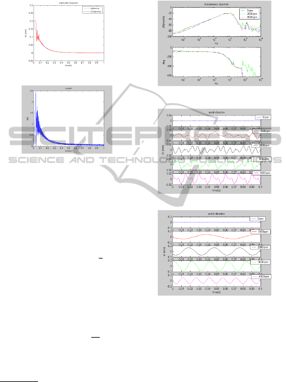
Figure 11: Transcient response of the axial displacement.
Figure 12: Transcient response of the coil current in the
active magnetic bearing.
the brushless DC motor is activated to spin the ro-
tor. The spinning test indicates that the rotor can
spin successfully to 4000rpm. Figure 13 shows the
disturbance rejection responses of the active bearing
for 0rpm, 2000rpm, and 4000rpm. The experimen-
tal setup for identifying these responses is the same
as what used in system identification except that the
input is changed to the disturbance signal. This fig-
ure indicates that the LTR controller renders the active
bearing fairly consistent disturbance-rejection perfor-
mance as the rotor speed varies. Particularly, the
static axial stiffness is greater than 10
7
N
m
, which ver-
ifies the high stiffness assumption in section 2. The
amplitudes of axial vibration and radial vibration
2
for
different spinning speeds are respectively shown in
Figure’s 14 and 15. It is clear that the bearings can
limit the rotor’s vibration to within one tenth and half
of the bearing gap respectively in axial and radial di-
rections. Moreover, according to Figure 15 the ra-
dial vibration is most significant between 2000rpm
and 3000rpm. This verifies the previous calculation
on the gyroscopic resonant frequency associated with
the designated tilting stiffness 18.02
N·m
rad
.
The radial vibration of the semi-active magneti-
cally levitated fan is also compared with two other
systems. One is the original fan in which mechani-
cal ball bearings are used to support the rotor, and the
other is the passive magnetic bearing system whose
2
The radial vibration is measured experimentally using a
laser displacement sensor.
Figure 13: Disturbance rejection responses of the active
magnetic bearing.
Figure 14: Steady state response of the axial displacement.
Figure 15: Steady state response of the radial displacement.
structure is similar to the current one except that the
active bearing is replaced by a mechanical thrust bear-
ing. The results of comparison are shown in Fig-
ure 16. Due to the gyroscopic resonance, the semi-
active system exhibits highest amplitude of vibration
between 1000rpm and 3000rpm. After 3000rpm, the
semi-active system’s vibration becomes smaller than
the passive one but still larger than the original fan.
In general, the vibration of the original fan is the low-
est among the three systems for Ω > 1000rpm. The
powerconsumption of these three systems are also ex-
perimentally compared and the results are plotted in
Design,AnalysisandControlofaSemi-activeMagneticBearingSystemforRotatingMachineApplications
509

Figure 17. It should be noted that while the power
in the semi-active system is consumed by the DC mo-
tor and the active bearing, the power for the other two
systems is solely consumed by the motor. As shown
in this figure, because the semi-active system is to-
tally frictionless and consumes almost zero-power in
levitation, it exhibits the lowest power consumption
among the three systems. Particularly, at the rated
speed the semi-active system consumes 14.7% less
than the original fan and 12% less than the passive
bearing system.
Figure 16: Comparision of the radial displacement for three
systems
Figure 17: Comparison of power for the three systems
6 CONCLUSIONS
In this paper, a semi-active magnetic bearing system
which incorporates both the active and passive mag-
netic bearings is proposed to support the rotor of an
axial fan. By carefully designing the radial stiffness
and tilting stiffness of the passivebearing and the con-
troller of the active bearing, the system can be suc-
cessfully operated to the rated speed with less power
consumption than the original fan. Currently, two
research efforts are conducted to further improve the
proposed system. One is to use inexpensive, small
hall-effect sensors to replace the expensive, bulky
fiber-optic sensor for positioning sensing. The other
is to modify the design of passive bearing I so that
it can be integraged with passive bearing II and be
placed internally. By doing so, the structural member
which mounts the magnetic ring and the senor can be
removed and the size, weight as well as the cost of the
semi-active system can be reduced.
ACKNOWLEDGEMENTS
The author gratefully acknowledges the support pro-
vided by Ministry of Science and Technology of Tai-
wan.
REFERENCES
Ansoft corporation, maxwell 3d, pittsburgh, pa, 2003.
Athans, M. (1986). A tutorial on the lqg/ltr method. In
Proc. American Control Conference, Seattle, WA.
H. Okuda, T. Abukawa, K. A. and Ito, M. (1984). Char-
acteristics of ring permanent magnet bearing. IEEE
Transactions on Magnetics, MAG-20(5).
J. Delamare, E. R. and Yonnet, J.-P. (1995). Classification
and synthesis of permanent magnet bearing configu-
rations. IEEE transactions on Magentics, 31(6).
J. Delamare, J.-P. Y. and Rulli, E. (1994). A compact mag-
netic suspension with only one axis control. IEEE
transactions on Magentics, 30(6).
J.F. Antaki, B. Paden, G. B. and Groom, N. (2000). Mag-
netically suspended miniature fluid pump and method
of designing the same.
J.F. Antaki, B. Paden, G. B. and Groom, N. (2001). Blood
pump having a magnetically suspended rotor.
K. Zhou, J. D. and Glover, K. (1996). Robust and optimal
control. Prentice Hall.
T.-J. Yeh, Y.-J. C. and Wu, W.-C. (2001). Robust con-
trol of multi-axis magnetic bearing systems. Interna-
tional Journal of Robust and Nonlinear Control, pages
1375–1395.
Yeh, T.-J., Chung, Y.-J., and Wu, W.-C. (2001). Sliding
control of magnetic bearing systems. ASME Journal
of Dynamic Systems, Measurement, 123(3):353–362.
Yonnet, J.-P. (1981). Permanent magnet bearings and cou-
plings. IEEE transactions on Magentics, 17(1).
ICINCO2015-12thInternationalConferenceonInformaticsinControl,AutomationandRobotics
510
