
Localization Method According to Collect Data from an
Acoustic Wireless Sensor Network
Example of Homarus Gammarus in Natural Area
Jean-Sébastien Gualtieri
2
, Bastien Poggi
1
, Paul-Antoine Bisgambiglia
1
, Thierry Antoine-Santoni
1
,
Dominique Federici
1
, Emmanuelle de Gentili
1
and Antoine Aiello
2
1
UMR SPE 6134, University of Corsica, Quartier Grossetti 20250, Corte, France
2
UMS Stella Mare, University of Corsica, Lido de la Marana 20290, Biguglia, France
Keywords: Localization, Acoustic Sensor, Method, Tracking, Position.
Abstract: The platform STELLA MARE (Sustainable TEchnologies for LittoraL Aquaculture and MArine REsearch)
has for objective to bring responses in the management of the sea in relation with the professional fishing. In
this paper, we introduce an experiment on the monitoring of Homarus Gammarus. Using a passive tracking
methodology using an acoustic wireless sensor network (AWSN), we try to follow some individuals, to
define movement. The main objective is to build a lobster path according to the collected signal according a
classical localization method to test our tracking method. Using a smoothing method and some resolution
algorithms we are able to deduct a behaviour of tagged lobsters in an experimental area. This paper
describes our methodology to estimate lobsters position according to data collected by an AWSN. This
work represent a first step before the building a lobster model to simulate its behaviour in Corsican
Mediterranean conditions.
1 INTRODUCTION
The global changes which affect the Earth have
more important consequences in closed spaces. It’s
the case of the Mediterranean Sea, and especially in
the island area. To relay in this subject, the
University of Corsica decides to create in 2010 the
platform STELLA MARE (Sustainable
TEchnologies for LittoraL Aquaculture and MArine
Research). This research center has been certified by
the CNRS, and the platform became the unit UMS
n°3514 Stella Mare University of Corsica/CNRS.
This unit is specialized in Marine and Littoral
Ecological Engineering. In this way, we have
selected, in interaction with the professional fishing,
species both studied in laboratories and in situ.
After a first experiment of Maja squinado
(Gualtieri, 2013) based only on an activity tracking,
we propose a second study of the Homarus
Gammarus. In Corsica, the population of Homarus
Gammarus is threatened and decreases strongly with
an impact also on the fishers’ activity. Stella Mare
wants to provide sustainable model for the lobsters
fishers in Corsican area. Indeed the distribution of
the target species can be affected by different
environmental conditions. However it is important to
collect data on the European lobster in Corsican area
because it doesn’t exist this kind of stud. These
works represent the first step before the building of
lobster model to simulate the behaviour of this
species. The European lobster, Homarus Gammarus,
has a broad geographical distribution. In its northern
range, it occurs from the Lofoten Islands in Northern
Norway to south-eastern Sweden and Denmark, but
is absent in the Baltic Sea probably due to lowered
salinity and temperature extremes.
Its distribution southwards extends along the
mainland European coast around Britain and Ireland,
to a southern limit of about 30 ̊ north latitude on the
Atlantic coast of Morocco. The species also extends,
though less abundantly, throughout the coastal and
islands areas of the Mediterranean Sea and has been
reported from the westernmost end of the Black Sea
in the Straits of Bosporus (Prodöhl, 2006).
According to our objective to build and simulate
a lobster model, we decided to track several
Homarus Gammarus using a VEMCO (VEMCO
Ltd, Nova Scotia) wireless sensor system to collect
33
Gualtieri J., Poggi B., Bisgambiglia P., Antoine-Santoni T., Federici D., de Gentili E. and Aïello A..
Localization Method According to Collect Data from an Acoustic Wireless Sensor Network - Example of Homarus Gammarus in Natural Area.
DOI: 10.5220/0005531100330041
In Proceedings of the 12th International Conference on Wireless Information Networks and Systems (WINSYS-2015), pages 33-41
ISBN: 978-989-758-119-9
Copyright
c
2015 SCITEPRESS (Science and Technology Publications, Lda.)

behaviour data. Acoustic telemetry systems are an
increasingly common way to examine the movement
and behaviour of marine organisms. However, there
has been little published on the methodological and
analytical work associated with this technology
(How, 2012).
Figure 1: Geographical distribution of Homarus
Gammarus (Prodöhl, 2006).
In this paper, we try to develop a simple way to
localize lobsters according to collected data from an
AWSN. In the first part of this paper, we present
several works on the lobster Homarus Gammarus
tracking. In the second part, we describe the material
and the used method to monitor the different
lobsters. We introduce our method to reconstitute a
position according to data collected by data
transceivers. The data collected are analysed in the
third part and the first results are shown. In part four,
we suggest the perspectives of this work and
expected results.
2 ACOUSTIC TELEMETRY AND
LOBSTER MONITORING
The acoustic telemetry is an important research area.
Indeed we can find an important volume of articles
of this problematic. In (Kilfoyle, 2000), the authors
explain that the acoustic telemetry channel is
bandlimited and reverberant which poses many
obstacles to reliable, high-speed digital
communications. In our study, we focus on lobster
monitoring using acoustic telemetry.
The north of the Europe is the main localization
of the most important studies on the Homarus
Gammarus. In south-eastern of Norway, the
Norvegian University of life science leads some
research on the lobster’s activities (Wiig, 2012). 50
males were tagged with acoustic sensors (VEMCO
V13). Tags were programmed to transmit signals (69
kHz) at 110 - 250 seconds random interval, equipped
also by a pressure sensitive sensor for the depth. To
follow lobster movement, 44 acoustic receivers were
deployed. The lobster’s beacons were able to
transmit a special signals for GPS data
reconstitution. This kind of research aims to identify
patterns of lobster movements through the use of a
sophisticated acoustic telemetry (AT) array which
will continuously map the movement of tagged
individuals, to within metres, within a large area
over several months. Improvements in AT now
allow us to tag and track large numbers of wild
lobster in situ with minimal amount of disturbance,
permitting studies which were previously impossible
using traditional techniques such as catch data, thus
improving quantification of movements, habitat
utilisation and zonation in a way that was previously
impossible (Skerritt, 2013). In (Moland, 2011), the
Florida wildlife research institute leads some
experiments with tagged a total of 10 lobsters in
May 2003, five males (mean ± SD: 95.8 ± 17.0 mm
carapace length, CL) and five females (80.6 ± 14.3
mm CL). The tags (VEMCO, V16 coded tags) were
16 mm in diameter, 58 mm long and produced a
coded signal in a randomised interval between 60
and 180 s. One year before deployment of receivers,
they conducted range tests of tags at Washerwoman
shoals. They defined that some rules to define the
position of lobsters according to the
detections/transmissions. This method allows them
to predict the lobster positon.
The precision of location estimates was
determined by the hourly centroids of a tagged
lobster that had entered a trap, which fell within a 30
m radius. The distance and velocity were estimated
using the Haversine formula. We can see that the
VEMCO low-cost solutions can represent a good
alternative for a quick deployment for an
experimental study (Heupel, 2006). It was precised
by the authors that the definition of the type of data
required will dictate the type of acoustic telemetry
the project requires and how best to deploy the
selected technology. The detection range is also
defined by the deployment of the receivers. In
(Simpfendorfer, 2008) the authors evaluated the
performance of receivers and explained that several
factors can affect the performance.
A large number of transmitters within the range
of receivers,
WINSYS2015-InternationalConferenceonWirelessInformationNetworksandSystems
34
A noisy environment,
A behaviour of the tagged animals,
The deployment method of the receivers,
The heterogeneity of the environment relative to
the transmission of acoustic signal (example:
estuarine area).
According to these different researches,
methodology and limits in the positions evaluation,
we defined an experimental area and we have
equipped 7 lobsters with VEMCO beacons. We
present the materials and method in the part III.
3 MATERIALS AND METHOD
3.1 Tracking Lobsters
For the tracking, we use VEMCO materials. During
this experiment, we have tagged 7 Homarus
Gammarus (male and female) with V13TP VEMCO
transmitters. The receivers are VEMCO VR2W
illustrated by the Figure 2 and 3. The research area is
near of Bastia city in Corsica. We can find a battle
wreck at a depth of 44 m. This area represents a
great zone for the lobster activities. We deployed 6
VEMCO receivers forming a grid around the wreck
showed by the Figure 4. This research area presents
two interests:
Signal analysis: the behaviour of the transmitters
– receivers of an AWSN in metallic
environment.
Biological: the behaviour of Lobster in special
environment (wreck).
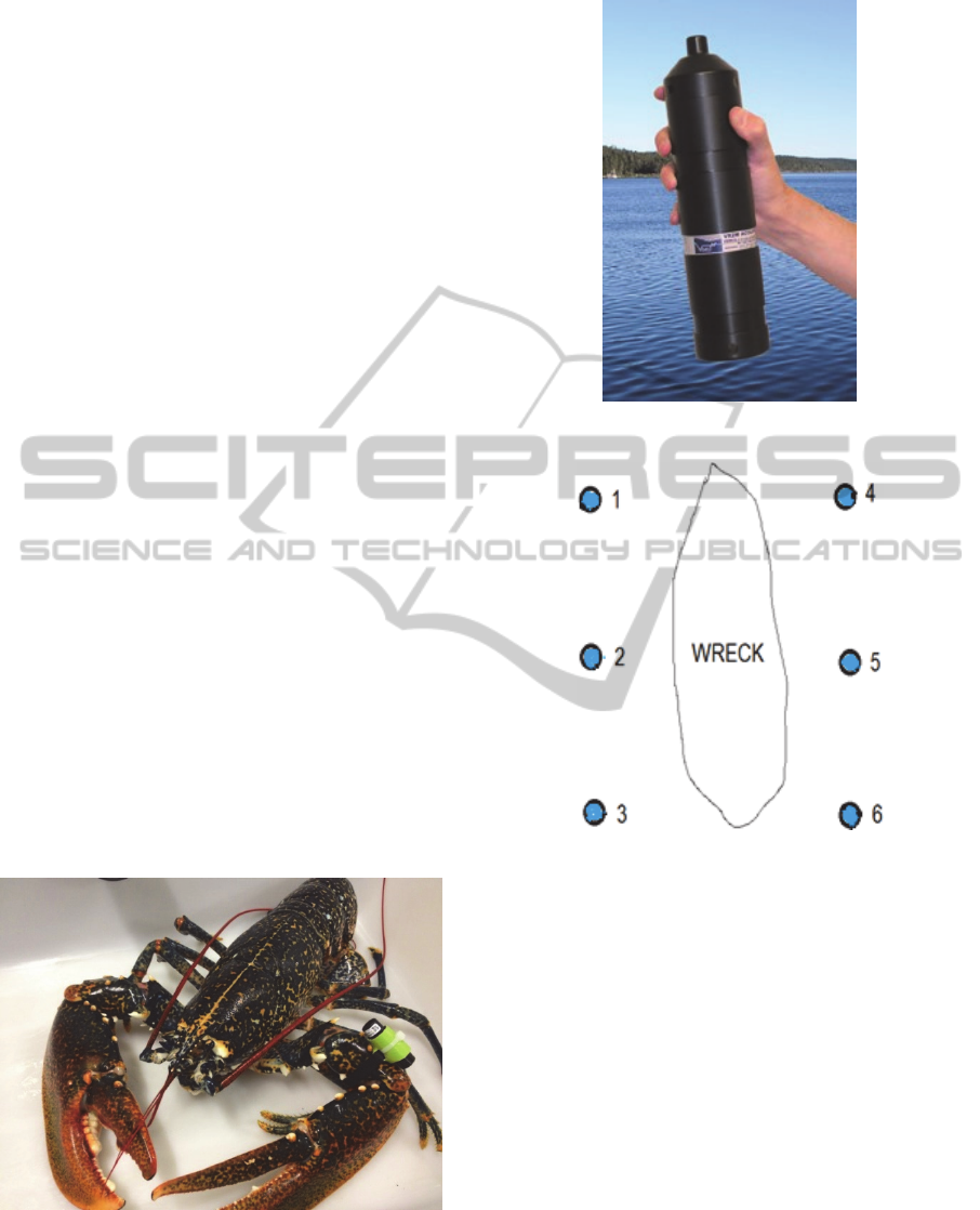
Figure 2: Hommarus Gammarus tagged with V13TP
VEMCO.
Figure 3: VR2W acoustic receiver.
Figure 4: Experimental area.
3.2 Noise Problem on Signal Reception
The collected data from the n=6 receivers
(hydrophone) (called Insuma 1 to Insuma 6) define
the presence of the different lobsters. The collected
data allow us to know if a lobster VEMCO signal
was received by the receivers. Each lobster can send
alternately two kinds of signals (ID Code):
temperature and pressure.
For the data treatment we group the two ID for
each lobster. In the deployment of two kinds of
beacons are deployed. The difference is on the
sampling frequency.
Transmitters 8788, 8790, 8792, 8794 et 8796
with a sampling frequency every 60 seconds
Transmitters 8798, 8800, 8002, 8804, 8806,
8810, 8812, 8814 and 8816 with a sampling
frequency every 90 seconds.
LocalizationMethodAccordingtoCollectDatafromanAcousticWirelessSensorNetwork-ExampleofHomarus
GammarusinNaturalArea
35

Several problems can disturb the signal reception:
If two beacons transmit at the same time a signal,
a collision can be created with information lost.
It is a reason of irregularity of the transmission.
A signal can be lost if a disturbance exists
between the lobster and the receiver.
A lobster can be invisible because there is an
obstacle between the V13TP and the VR2W.
According to these different researches,
methodology and limits in the positions evaluation,
we defined an experimental area and we have
equipped 7 lobsters with VEMCO transmitters.
3.3 Method to Deduct Position
According Data Collected
In this part, we present the used method to deduct
lobster position according data collected. We use
classical methods, described more precisely in the
3.3.2. Indeed, the objective of this work was to have
a simple method to have lobster position
independent of VEMCO systems and manufactures,
based only on the received signals integrating a
possible development way towards a real time
analysis.
The first analyze of the data collected allows us
to have a presence or not of a signal (of a lobster) on
the different receivers as showed on our example in
the Figure 5 during a day.
Figure 5: Data collected by the 6 deployed receivers for a
day and a tagged lobster 8798 (y = receivers VR2W (1 to
6) and x= Time of arrival of a message on a receivers).
We see that the possible noise of the
environment and the possible loss of signals could
be explained by the experimental metallic area of the
wreck. We can estimate that it is a first result,
clearly different of our first tracking activity
(Gualtieri, 2013). The reception of message is
clearly dependant of the distance between a lobster
and a receiver. To remove the noise we use a
smoothing method according to Savitzky-Golay
algorithm. According to the smoothed data we
present a method to deduct the localization of the
lobster and a global behavior.
3.3.1 Smoothing Method
On the Figure 5 we can observe the data collected
for tagged Lobster 8798.
In each point x of the Figure 5, we treat the curve
as a polynomial P(t) in order d with d <2L+1. L is
the window of values.
̅
⋯
In the point x-L,…, x, x+L the polynomial must
coincide with the values of the function to smooth. If
we center the resolution in 0, i.e. by setting x = 0, a
set of equations is obtained to resolve –L, ...1 , 0 , 1,
...L. The ɑ
0
value corresponds to the smoothed value
x ɑ
1
and its derivative.
..
..
1
.. ..
..
.. ..
1
.. ..
1
..
.. ..
..
∗
..
The Figure 6 shows the smoothed curved. The
effectiveness of a smoothing increases with the
number of points considered, the dispersion values is
reduced. After smoothing the error on the points
decrease as much as the convolution involves a large
number of points.
Figure 6: Smoothed curve according to Figure 5.
If we do not wish to have access to different
derivatives, it is not necessary to choose a high
degree for the polynomial. For a polynomial of
degree 3 and a window of size L = 10 are obtained.
3.3.2 Localization Method
To determine the position of individuals in relation
to the stations, we need to receive functions R. It is
assumed that the reception is not oriented, and it
depends only on the distance D of the individual
from the station. In this case, it is inversely
proportional to the distance, which we estimate
based on a distance -related exponential D.
,
,
With
,
WINSYS2015-InternationalConferenceonWirelessInformationNetworksandSystems
36

R is the reception rate; R
max
is the maximum value
of R (100). N
0
is a starting constant to receive curve
(the higher this value is small and the curve will
remain longer in the vicinity of R
max
for small values
of D. r is a damping coefficient. On the Figure T we
can distinguish the impact of r on the R receives
functions. According this parameter r, we can
describe the derived functions.
,
,
,
,
1
,
,
1
To find the position of an individual at time t, we
will minimize the quadratic error in measuring the
difference between the R function (x, y) and the
measures taken at the time t.
,,
̅
,,
δ(x, y, t) is the error to be minimized.
i
correspond
to the smoothed values for each station.
the
weights of each measure The idea is from a point
,
to calculate a new point
,
which decreases the value δ. At each
iteration, we calculate η a disturbance that will
evolve the squared error to a minimum.
The gradient descent algorithm allows to find the
minimum. In this case the disturbance occurs in the
direction of the steepest gradient provided by
,
,. The disturbance η
dg
that minimizes δ
2
is
found when de gradient of the squared error is null.
2
̅
0
̅
Where W is the weighting matrix with
1/
,
and J is the Jacobian matrix.
This algorithm is simple to implement, but the
starting point should be close to the global
minimum. With a not too large step the method can
quickly become chaotic, whereas with a not too
small step this method can be very long and
converge to a local minimum. The η
dg
perturbation is
proportional to previous described value, where the
positive scalar determines the length of the step in
the steepest-descent direction. It is possible to
change this value by increasing or decreasing it
when the error decreases or increases.
The Gauss-Newton method is a well-known
iterative technique used regularly for solving the
nonlinear least squares problem (NLSP) (Press,
1992). This method is more stable than that of the
gradient, it allows to converge in most cases. We
approximate the δ(x, y, t) by a quadratic function in
the vicinity of the solution, which avoids using the
Hessian of R
i
. That is to limit the development R
i
to
the first derivative.
If we inject the value of R in p
j
to calculate the value
of the square error p
j+1
gives an estimate of the
derivative of
,
,.
2̅
2
And when squared error is null we can obtain the
local disturbance.
̅
The Levenberg-Marquardt (LM) algorithm is an
iterative technique that locates the minimum of a
function that is expressed as the sum of squares of
nonlinear functions (Levenberg, 1944), (Lourakis,
2005), (Marquardt, 1963). It has become a standard
technique for nonlinear least-squares problems and
can be thought of as a combination of steepest
descent and the Gauss-Newton method.
̅
The disturbance corresponds is given by the
equation. If λ tends to 0 we approach the Gauss-
Newton method and so λ is more important we
approach the gradient descent algorithm. At the start,
we will fix a λ value that will decrease as the square
error increases. This value will increase as soon as
the square error decreases, to be closer to the
gradient method.
The following algorithm is used to compute the
optimal solution of the squared error between
collected data and the receive functions R. The
Levenberg Marquardt algorithm (Nocedal, 1999),
(Kelley, 1999) requires an initial value for
to be
estimated at t time. We chose
equal to
evaluate at the previous time (the last position of the
lobster). When the lobster is hidden, this position is
not available, so we use the latest known position.
This algorithm computes the disturbance and
evaluates the error at the new parameter vector. If
the error has increased as a previous result,
is
increase by a factor of 10, and the step is rejected. If
the error has decreased as a result of the update we
LocalizationMethodAccordingtoCollectDatafromanAcousticWirelessSensorNetwork-ExampleofHomarus
GammarusinNaturalArea
37
accept the step and decrease
by a factor of 10. We
stop the steps when the algorithm met the desired
convergence criteria or has exceeded the limit of
function evaluations or iterations.
Algorithm.
for each time t
{ initialization of
;
choose
=max
,
and
continue=true ;
while (continue and iteration<limit)
{ Compute the new disturbance
Evaluated the new squared error
if
‖
‖
‖
‖
continue=false;
else
{ evaluate an acceptability factor
‖
‖
‖
‖
2
̅
if (
0)
; decrease
;
else increase
;
}
iteration = iteration +1;} }
and limit are user specified.These methods were
implemented in C# and the treated data are
presented on the following figures.
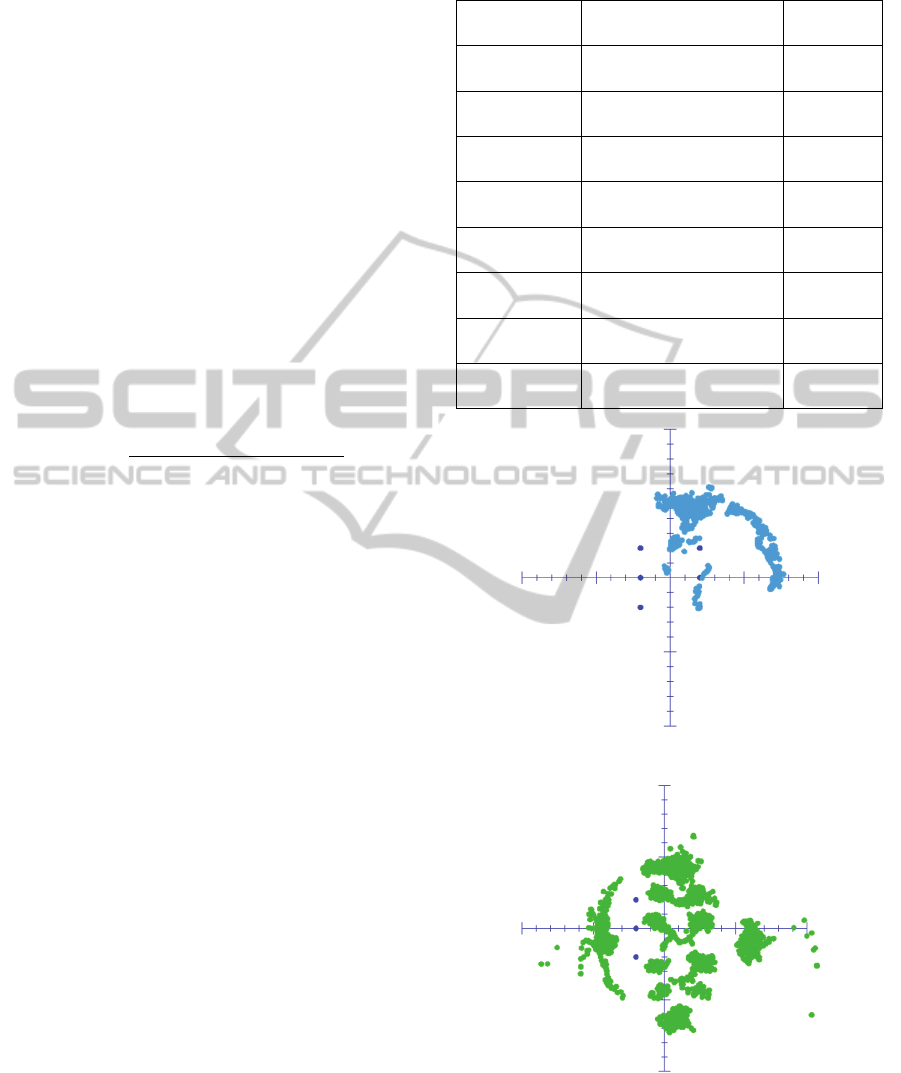
4 RESULTS
In this part we present the activity of each tagged
lobster after position calculation according to the
previous methods.
On the presented figures we can see only a static
activity. It is important to precise that we have an
activity monitoring step by step. On the different
figures we can observe the blue points which
represent the experimental area as showed on the
Figure 4. On the table 1 we introduce the monitoring
period for each lobster that corresponds at the usable
collected data are.
We can observe on the different figures that we
are able to distinguish an activity for each observed
lobster. The signal loss can appear on different
figures (Figure 7 and Figure 14).
Table 1: List of figures.
Lobster
Period
(0h00 to 0h00)
Figure
8794
6 June 2014 to 27 June
2014
Figure 7.
8798
17 September 2014 to 5
th
January 2015
Figure 8.
8806
17 September 2014 to 12
October 2014
Figure 9.
8812 6
th
June to 12 August 2014 Figure 10.
8812 (bis)
14 August to 1
st
October
2014
Figure 11.
8814 6
th
June to 12 August 2014 Figure 12.
8816 6
th
June to 12 August 2014 Figure 13.
8816 (bis)
14 August to 1
st
October
2014
Figure 14.
Figure 7: Activity of tagged lobster 8794.
Figure 8: Activity of tagged lobster 8798.
WINSYS2015-InternationalConferenceonWirelessInformationNetworksandSystems
38
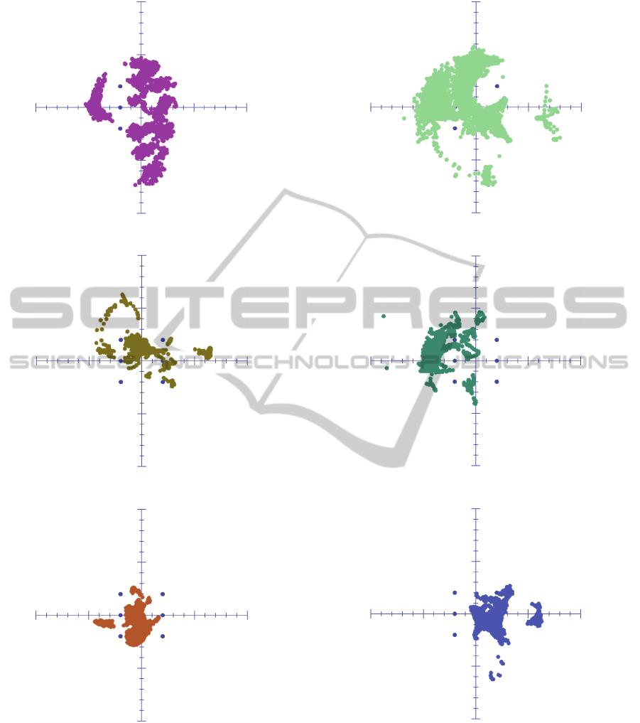
Figure 9: Activity of tagged lobster 8806.
Figure 10: Activity of tagged lobster 8812.
Figure 11: Activity of tagged lobster 8812 (bis).
These figures show that the used method allow
us to deduct a behaviour during a period according
collected data using a subaquatic wireless sensor
network.
Figure 12: Activity of tagged lobster 8814.
Figure 13: Activity of tagged lobster 8816.
Figure 14: Activity of tagged lobster 8816 (bis).
It is important to precise the collected data is
dependant by the capacity of the receivers to receive
the signals. Indeed the activity of the lobster is
clearly is diurnal and during the day the lobster is in
its habitat, in a metallic area with an important
impact on the signal transmission. The figures show
only the behaviour during the night corresponding at
the hunt behaviours of the lobsters. During, the
LocalizationMethodAccordingtoCollectDatafromanAcousticWirelessSensorNetwork-ExampleofHomarus
GammarusinNaturalArea
39

lobster leaves its habitat and allows a new
transmission of the Vemco units. The wreck is rich
in foods and we can observe a stillness of the
lobsters. When the lobster leave the wreck we can
observe a loss of signals because the research area is
limited by 6 receivers and the distance between
transmitters – receiver is too important.
5 CONCLUSIONS
These results show that the used method allow us to
deduct a behaviour during a period according
collected data using a subaquatic wireless sensor
network. The monitoring of Homarus Gammarus in
the Mediterranean Sea can play an important role on
the economic development of sustainable fisheries
activity. In this context, this paper want to provide a
simple way to predict the behaviour of this species
according collected data by an acoustic wireless
sensor network.
This paper presented a part of the state of art on
the monitoring of Hommarus Gammarus using a
passive tracking with an acoustic wireless sensor
network from VEMCO technology. According to the
data collected we tried to define the position and the
global behaviour of 7 tagged lobsters. We can see
that we are able to build a global behaviour of the
lobsters from collected signal. This behaviour
building is deducted from classical localization
method. This method is a hybridization of two
classical methods. Indeed, according to a given
value λ we use either gradient descent or Gauss
Newton method.
The goal of this study was not to develop a new
method of localization but to build a simple way to
deduct from collected data the relative position of
the tags and to extract a behavior. In this experiment,
the results are generally positive but not sufficient.
Indeed we are able to have a position but we are not
sure of the precision. The impact of the damping
coefficient r must be measured and reported in our
estimation of the position. We must a measurement
campaign during a year to observe the complete
behavior of a lobster.
The impact of receiver’s positions must be better
appreciate. Indeed we made the choice to deploy the
VR2W in the fund of the sea however it seems to be
more precise to deploy under the sea surface to
improve reception quality. The choice of the
research area (wreck with metallic body) has an
impact on the signal.
However these first results allow us to build a
first behavior model of individual lobster according
to the collected and interpreted data form the sensor
network in the Mediterranean Sea. Indeed the
diurnal activity, the stillness of the lobster on a rich
foods area are the first elements of a corsican lobster
behavior to find some solutions in the repopulation
of this species.
ACKNOWLEDGEMENTS
We thank the team of aquaculture technicians of
Stella Mare platform for their assistance in the
capture and the tagging of lobsters. We also thank
the divers’ team of recover the submerged
hydrophones and allow us to collect monitoring
data. Thanks to: Romain Bastien, Sébastien
Quaglietti, Jérémy Bracconi, Nicolas Tomasi,
Michel Marengo and Jean-José Filippi.
We also wish to thank ML Bégout of the
IFREMER of La Rochelle to have lent us the
hydrophones that were used for this experiment.
REFERENCES
Gualtieri, J. S., Aiello, A., Antoine-Santoni, T., Poggi, B.,
& De Gentili, E. (2013). Active Tracking of Maja
Squinado in the Mediterranean Sea with Wireless
Acoustic Sensors: Method, Results and Prospectives.
Sensors, 13(11), 15682-15691.
Prodöhl, P. A., Jørstad, K. E., Triantafyllidis, A., Katsares,
V., & Triantaphyllidis, C. (2006). European lobster-
Homarus gammarus. Genetic Impact of Aquaculture
Activities on Native Populations. Final Scientific
Report, 91-98.
How, J. R., & de Lestang, S. (2012). Acoustic tracking:
issues affecting design, analysis and interpretation of
data from movement studies. Marine and Freshwater
Research, 63(4), 312-324.
Kilfoyle, D. B., & Baggeroer, A. B. (2000). The state of
the art in underwater acoustic telemetry. Oceanic
Engineering, IEEE Journal of, 25(1), 4-27.
Wiig, R., Jorgen, (2012), Acoustic monitoring of lobster
(Homarus Gammarus) behaviour survival during
fisheries, Master Thesis.
Skerritt, D.J., Fitzsimmons, C., Hardy, M.H., Polunin,
N.V.C. (2013) Mapping European lobster (Homarus
gammarus) movement and habitat-use via acoustic
telemetry – Implications for management. Progress
report to the Marine Management Organisation. Oct
2013.
Moland, E., Olsen, E. M., Andvord, K., Knutsen, J. A., &
Stenseth, N. C. (2011). Home range of European
lobster (Homarus gammarus) in a marine reserve:
implications for future reserve design. Canadian
Journal of Fisheries and Aquatic Sciences, 68(7),
1197-1210.
WINSYS2015-InternationalConferenceonWirelessInformationNetworksandSystems
40

Heupel, M. R., Semmens, J. M., & Hobday, A. J. (2006).
Automated acoustic tracking of aquatic animals:
scales, design and deployment of listening station
arrays. Marine and Freshwater Research, 57(1), 1-13.
Simpfendorfer, C. A., Heupel, M. R., & Collins, A. B.
(2008). Variation in the performance of acoustic
receivers and its implication for positioning algorithms
in a riverine setting. Canadian Journal of Fisheries and
Aquatic Sciences, 65(3), 482-492.
Lourakis, M. I. (2005). A brief description of the
Levenberg-Marquardt algorithm implemented by
levmar. Foundation of Research and Technology, 4, 1-
6.
Press W, Teukolsky B.F.S, & Vetterling W. (1992)
Numerical Recipes: The Art of Scientific Computing.
second ed. Cambridge: Cambridge University Press;
1992.
Levenberg, K. (1944) A Method for the Solution of
Certain Non-linear Problems in Least Squares.
Quarterly of Applied Mathematics, 2(2):164–168, Jul.
1944.
Marquardt D. (1963) An algorithm for least squares
estimation of nonlinear parameters. J Soc Ind Appl
Math 1963;11:431–441.
Nocedal J. & Wright, S. (1999) Numerical Optimization.
Springer, New York, 1999.
Kelley C. (1999) Iterative Methods for Optimization.
SIAM Publications, Philadelphia, 1999.
LocalizationMethodAccordingtoCollectDatafromanAcousticWirelessSensorNetwork-ExampleofHomarus
GammarusinNaturalArea
41
