Calibration of Laser Range Finders

for Mobile Robot Localization in ITER

Tiago Sousa

, Alberto Vale

and Rodrigo Ventura

Instituto Superior Técnico, Universidade de Lisboa, Av. Rovisco Pais 1, 1049-001, Lisboa, Portugal

Instituto de Plasmas e Fusão Nuclear, Instituto Superior Técnico, Universidade de Lisboa,

Av. Rovisco Pais 1, 1049-001, Lisboa, Portugal

Laboratório de Robótica e Sistemas em Engenharia e Ciência, Instituto Superior Técnico, Universidade de Lisboa,

Av. Rovisco Pais 1, 1049-001, Lisboa, Portugal

Keywords:

Laser Range Finder, Calibration, Localization, ICP.

Abstract:

Remote maintenance operations in the experimental fusion reactor ITER may require vehicle localization, for

which one of the proposed methods is based on a network of Laser Range Finder sensor measurements. This

localization method requires an accurate knowledge of each sensor pose (position and orientation). A deviation

in sensor pose can compromise localization accuracy thereby recalibration procedure for the sensor poses is

often necessary. This paper studies several calibration algorithms based on ICP. Simulation and experimental

tests were carried out for different maps and situations regarding sensor pose uncertainty. The conclusion

proposes the best suited algorithms for each scenario.

1 INTRODUCTION

Producing enough energy to cover our civiliza-

tional primary energy needs and living standards, has

always been one of the main goals and focuses of our

modern civilization. The current growth in energy

supply demand has raised the concern on the environ-

mental impact of current ways of energy production

and lead to the discussion of reliable and new alter-

natives. Fusion power promises itself as a clean, and

sustainable source of usable energy. The biggest chal-

lenge now is to prove that a large scale functionality

and production is possible. The International Ther-

monuclear Experimental Reactor (ITER) is a multi-

national in-progress experimental project located in

Cadarache, south of France and represents the next

step of demonstration. Workers are not allowed to en-

ter the ITER facilities during its operation and trans-

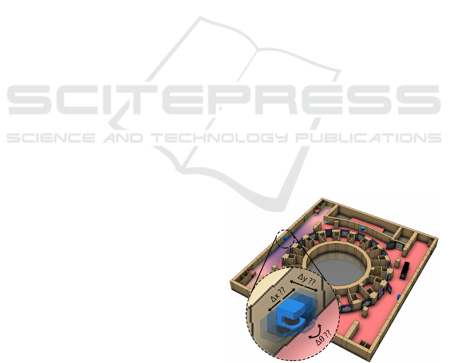
portation of activated components (see Figure 1).

Instead, the nominal and maintenance operations

(A. Tesini, 2008) will be handled completely re-

motely. Some of the critical operations include the

transportation of shielded casks, that enclosures the

load and spare parts by the Cask and Plug Remote

Handling System (CPRHS) vehicles and Cask Trans-

port System (CTS) (Darren Locke, 2014) vehicles and

the operation of rescue vehicles such as the proposed

Multi Purpose Rescue Vehicle (MPRV) (J. Soares,

Figure 1: Problem illustration in ITER building.

2014) for inspection, repair and component replace-

ment. To perform the previous and other tasks with

minimal error margin, an accurate navigation method

is needed due to the tight safety margins inside the

building. The navigation uses the vehicles localiza-

tion estimation (J. Ferreira, 2013) to autonomously

maneuver the vehicle trough its path or to help a hu-

man operating it remotely. A network of Laser Range

Finder (LRF) sensors are proposed, due to their im-

munity to magnetic ﬁelds that proliferate in near the

Tokamak and high accuracy distance measurements

541

Sousa T., Vale A. and Ventura R..

Calibration of Laser Range Finders for Mobile Robot Localization in ITER.

DOI: 10.5220/0005536505410549

In Proceedings of the 12th International Conference on Informatics in Control, Automation and Robotics (ICINCO-2015), pages 541-549

ISBN: 978-989-758-122-9

 2015 SCITEPRESS (Science and Technology Publications, Lda.)

in long and short distances, which the localization es-

timation method is based and heavily reliant on.

Calibration is a problem that relies on most of the

sensors, in particular, the ones used in high demand-

ing accuracy applications. After the ﬁrst calibration,

every sensor might need a recalibration depending on

some working condition factors such as level of tear,

stability and wear suffering during operational time.

Besides the general problems in calibration regard-

ing sensor’s own measurements, here the focus is on

calibrating the measurements between a network of

LRF sensors in such a way the measurements from

different sensors could have a valid correspondence

between them (see Figure 1). The devices are attached

to environment walls to reduce the chance of elec-

tronics being damage by the radiation. A deviation of

100 mm in sensor position and 5

◦

in orientation could

cause as much as a deviation of about 120 mm (as

stated in (J. Ferreira, 2013)) and 873 mm respectively

in vehicle location. These deviations compromise ma-

neuvers of hazard material transportation vehicles on

narrow and tight spaces.

LRF sensors have becoming of widespread use in

mobile robot systems because of its high accuracy

distance measurements. Among LRF, other sensors

such as cameras (IR and RGB) and odometry infor-

mation are often used simultaneously to guide au-

tonomous vehicles. Some methods for calibration be-

tween a camera and LRF have been proposed (Vin-

cenzo Caglioti, 2008), other methods such as SLAM

(Sebastian Thrun, 2008) use the odometry informa-

tion along LRF readings in its localization algorithm.

In the previous approach, after calibration, the results

are given in the robots frame which is not static, so the

readings might change with time. In ITER sensors are

ﬁxed to environment walls. When calibration proce-

dure takes place, it is assumed that all measurements

are derived from the map so no ﬁx or moving outliers

presence were considered. The only changes in LRF

consecutive measurements should be associated with

the sensor precision limits.

Some LRF calibration techniques have been

proposed such as (Antone and Friedman, 2007),

(K. Schenk, 2012) but all of them have one thing in

common: they require physical access to the environ-

ment where the calibration takes place. Since no hand

calibration is possible, the calibration procedure, like

many other operations in ITER context, must be made

entirely remotely. The Calibration techniques stated

before, use static or moving objects (or humans) that

must be asymmetrical to uniquely identify the target.

That is not the case as the CTS vehicle features a sym-

metrical rectangular shape and uses a rhombic-like

kinematics conﬁguration for high maneuvering and

ﬂexibility making heading extraction not trivial.

Given the physical access constraints of ITER, a

map description of the environment shall provide the

valuable opportunity to check and compare where the

LRF measurement data best ﬁts on the map. There-

fore the map layout description should be as accurate

as possible to mitigate the impact of erroneous walls

dimensions or unmapped areas/objects on results.

This paper is divided as follows: Section 2

presents the proposed solution. The implemented

simulation environment is described in Section 4, pre-

ceded by the obtained results in Section 5. Finally, the

last section is reserved for the conclusions discussion.

2 PROBLEM STATEMENT

In ITER, the optimal locations where the LRF sensors

should be installed are determined beforehand by an

algorithm in (J. Ferreira, 2013). As a consequence

of sensor misplacement, measurements from distinct

LRF lose correspondence between them. Address and

solving this problem is the main focus and objective

of the present work. This issue, where the exact posi-

tion and orientation of the sensors are spoiled, can be

caused by human error on installation procedure, er-

roneous map measurements or any other factor such

as the ones mentioned in Section 1.

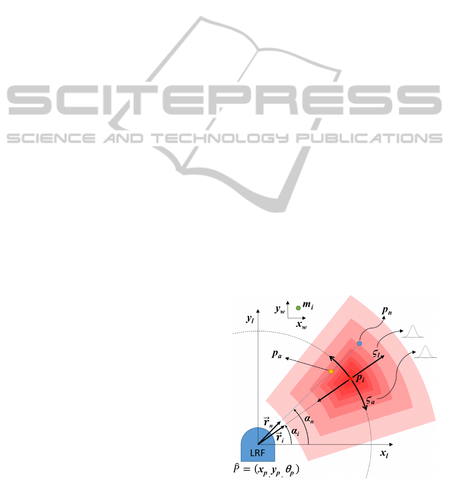
The pose P, for a given sensor in the network, in-

cludes its position coordinates (x

) in meters and

its orientation θ

in angle degrees. Both are given

in the map coordinate frame (x

) as illustrated in

Figure 2. Also a horizontal orientation is assumed

(pitch and tilt not inﬂuential).

Figure 2: Variables involved in the problem description.

ICINCO2015-12thInternationalConferenceonInformaticsinControl,AutomationandRobotics

542

The LRF sensors return data in two dimensional polar

coordinate system where the distance measurements

and the associated angle α

are given in device

frame (x

). Since the distance measurements are

affected by noise, LRF returns

measurements in-

stead of the true

yielding the p

points. The ob-

jective is to estimate the absolute ﬁnal pose,

, of

each sensor in the network that minimizes the mean

quadratic error, e

, function in (1). The residual is

composed by the point to point Euclidean distance be-

tween the transformed LRF measurements T (

, p

)

and the respective map closest points m

. This is a dif-

ﬁcult optimization problem due to several local min-

ima existence.

= argmin

∑

kT (

, p

) −m

(1)

3 PROPOSED SOLUTION

The proposed solution is a main algorithm that re-

ceives as input a map description, LRF measurement

data, and an optional initial pose estimate

. The un-

certainty degree associated with this parameter leads

to four different scenarios (denoted A, B, C, and D

below) that specify the way the algorithm behave. In

case an initial pose estimate is given (scenario A), the

algorithm behaves locally trying to extract the best

pose for the given measurements. Instead, if an ini-

tial pose estimate is not given at all (scenario D), the

algorithm behaves globally on the map, assuming any

pose is plausible. Other two intermediate scenarios

(B, C) may occur whenever one parameter of the ini-

tial pose is missing.

3.1 Data Pre-processing

This ﬁrst phase in the algorithm execution is common

in every case scenario. By averaging raw data from

multiple scans, it is possible to mitigate the errors in

readings derived from the random errors in LRF de-

vices. This way precision improves proportionally to

the square root of the number of complete scans as

stated in (Markus-Christian Amann, 2000). But be-

fore averaging, a normality test takes place to verify

if data its well a modeled normal distributed popu-

lation so an averaging metric could be meaningful in

this context. The averaging method implemented uses

a signiﬁcant number of scans (at least one hundred) to

determine the average value µ, and the standard devia-

tion σ. Using a window interval, w, given by (2) it was

possible to reject the extreme values before applying

the average metric. As average metric is strongly in-

ﬂuenced by extreme values, and after some experi-

mentation, only the values inside of σ range (68%)

were considered to reduce this negative effect.

w = [µ − σ,µ + σ] (2)

3.2 A: Initial Pose Known

In this case, an initial pose estimate (position and ori-

entation) is completely known, and, therefore, a local

based search is performed using LRF readings against

the map. In order to match the data type returned

from LRF readings (Cartesian points), the map line

segments need to be transformed into a signiﬁcant

number of points to preserve data integrity as much as

possible. The origin of the LRF points are translated

to the given position coordinates and rotated accord-

ing to the given orientation. Then, a matching pro-

cedure takes place to adjust and align the LRF points

with the map points to determine the best ﬁtting pose.

To match the two point clouds and evaluate the dis-

placement error, the Iterative Closest Point (Besl and

McKay, 1992) (ICP) algorithm, represented in (3),

was used.

= argmin

R,t

∑

kRp

+t − m

(3)

The map points, m, are chosen as the reference and

LRF points, p, are subject to a rigid body transfor-

mations R,t that aligns the two by minimizing the

quadratic error of the point to point distance metric at

each k iteration for the all the N LRF points. The algo-

rithm stops when the point association between the k

and k −1 iterations are the same. The resultant output,

and t

, is the rigid body transformation that best

ﬁts the two point clouds and is determined from SVD

decomposition (K. S. Arun, 1987). By applying the

result to the initial guess the ﬁnal pose estimate is re-

vealed. One major drawback in this algorithm is that

the ICP can be trapped in local minima and this is the

main reason why it has been chosen for local search

scenario. Variations of this algorithm that matches

points to lines such as (Low, 2004)and (Censi, 2008),

have been proposed but the error metrics require non

linear minimization metrics which are solved using

approximations and are not robust against large initial

displacement error. Point to point metric presents a

closed form solution and converge faster despite time

not being a priority in the context of this application.

If the solution presents an associated error with a or-

der of magnitude higher than the devices standard de-

viation (STD), the initial pose estimate was not good

enough therefore other case scenarios are applied. In

these other scenarios where the initial pose estimate

is incomplete or non-existent, the resultant pose esti-

mate always suffer a ﬁnal ICP alignment.

CalibrationofLaserRangeFindersforMobileRobotLocalizationinITER

543

3.3 B: Only Position Known

In this case only a position initial estimate is known.

Taking advantage of the available information, the

proposed solution consists in a brute force approach

of the previous scenario. Thus the ICP algorithm is

initialized for a predeﬁned set of poses where only

the estimate orientation angles vary. The chosen ori-

entation values should be as low as possible apart so

the ICP algorithm has a higher chance to converge to

the optimum solution without being stuck in a local

minima. The ﬁnal estimated pose is given by the pose

with the lowest ICP associated e

3.4 C: Only Orientation Known

When only the orientation initial estimate is given,

again, a brute force version of ICP could be applied

varying the position, but depending on the point den-

sity of the map, the successive ICP could become very

computationally heavy. As an alternative, a novel

method was developed consisting in using the read-

ings as a projection of the possible location of the

sensor. Every single LRF measurement is projected

backwards from each map point revealing a LRF pos-

sible location. A vote is then accumulated for the re-

spective coordinates. The coordinates which have a

higher vote count determines the most likely position

estimate.

3.5 D: Initial Pose Unknown

This is the worst case scenario as the LRF location

can be anywhere in the map. In order to reduce the

search space, when compared to the previous solu-

tions, a different approach was taken. The method

presented does not taken into account the wall instal-

lation constrain and is divided into two phases: fea-

ture extraction and matching features. A ﬂowchart

is provided on Figure 3, which depicts the following

different phases and main steps involved in this case

scenario.

Figure 3: Flowchart of scenario D.

3.5.1 Feature Extraction

The objective in this phase is to extract line segments

and vertex points from the processed LRF output data.

A comparison between some of the most common

line extraction methods is present in (Viet Nguyen,

2007). Based on the conclusions, the most correct and

best suited method for the localization problem with

an a priori map was the Split and Merge technique

preceded by a clustering algorithm. So the ﬁrst step

is to perform a primary classiﬁcation of points using

a clustering technique. The Distance based Convolu-

tion Clustering (DCC) proposed by (Carlos Fernán-

dez, 2010) was used. It consists on identifying break

points based on a sudden change of the distance be-

tween consecutive scan points, and once one is found

a new cluster is created. To do that, a high pass ﬁlter is

applied to the set of euclidean distances between con-

secutive points. The break points are identiﬁed where

the convolution is greater than a cluster threshold

whose value is proportional to the LRF readings stan-

dard deviation. Wrong or missing breakpoint identiﬁ-

cation can happen as this is a simple and primary ap-

proach. The following step uses the Split and Merge

algorithm to conﬁrm and correct for those erroneous

cases in order to ﬁnally extract lines and vertex points.

The Split and Merge technique begins by the splint-

ing phase where the objective is to create sub-clusters

of a cluster based on the evidence of a line pattern

points. A line ﬁts the points using an ordinary least

squares line ﬁtting technique and a breakpoint is iden-

tiﬁed if the most distant point to the line is greater than

a given split threshold. Since the previous procedures

can wrongly create more than one line segment for the

same correspondent line in the map, a merging phase

is conducted to unify similar clusters. If two neighbor

segments have its respective, angle difference inferior

to a given slope threshold, and distance between two

extreme points inferior to a proximity threshold, the

two respective clusters are uniﬁed. The segment line

parameters, for this uniﬁed cluster, are extracted, this

time, using a M estimator robust line regression tech-

nique with a bi-square weight function. Vertex points

are extracted extending and intercepting consecutive

and close enough line segment extremes.

3.5.2 Feature Matching

The matching phase takes advantage of the geometric

features extracted previously, specially the vertexes.

An extraction of map vertexes is ﬁrst performed, and

then, a matching hypotheses is formed for every pair

combinations of map vertexes and extracted vertexes.

Assuming a vertex is the common extreme point of

two different line segments, after overlapping the two

vertex points in the pair by a translation transforma-

tion means, there exists a four possible pair combi-

nations of alignments for the vertexes respective line

segments. This alignments are done by means of rota-

ICINCO2015-12thInternationalConferenceonInformaticsinControl,AutomationandRobotics

544

tions. The extracted rigid body transformation is ap-

plied to all LRF points and after this transformation

the pp error function in (1) is used to assess and eval-

uate the displacement between the two point clouds.

The resultant estimated pose,

, is determined from

the transformation that yields the lowest error. In case

no vertexes are extracted, threshold values that af-

fect the feature extraction phase are changed and the

procedure is repeated. If the combinations of tested

threshold values are not enough to produce a valid re-

sult, i.e., a result whose the point to point error value

is relatively close to the devices standard deviation, an

extremes matching method is applied. This method

procedure is similar to the vertex method except it

uses end points of extracted line segments instead of

vertexes. For every pair of points (one map vertex and

one end point from an extracted line) a two combina-

tion matching (instead of four) is done by aligning the

line segment with the two map lines that originate the

map vertex in question.

4 SIMULATED RESULTS

4.1 LRF Simulation

To test and conﬁrm the proposed solution, a simulator

was developed which is composed by two parts: the

LRF model and LRF scan procedure. The two are in-

timately linked as the model contains the device prop-

erties that inﬂuence the scan result. Noise source, in

LRF devices, mostly comes from internal electronics

generating jitter, walk nonlinearity, and drift (Markus-

Christian Amann, 2000) which affect sensor accuracy

not only by distance reading means but angular steps

also suffer from deviation despite being almost in-

signiﬁcant. To simulate noise, a normal distribution,

with zero mean and standard deviation given by man-

ufacturer, was chosen to model the deviation from the

correct value, p

. This point is obtained in the simu-

lator by intercepting every sensor ray with every wall

and selecting the appropriate point. The coordinates

of a point affected by noise, p

, is given by (4).

= T

(ζ

) ∗(p

(ζ

,~r

)) (4)

It should be noted that linear and angular noise are

not commutative operations due to the nonlinearity of

map. That being said, ﬁrst, the p

is obtained from

provoking an angular deviation ζ

to ~r

yielding ~r

Then T

(ζ

) applies a linear deviation of ζ

in the di-

rection of ~r

(see Figure 2). A value for the LRF range

parameter is often given by the manufacturers under

certain ideal conditions and a range correction factor

is often provided to compensate for changes of these

conditions. For simulation purpose meteorologic con-

ditions are assumed ﬁne with no inﬂuence on read-

ings. The target reﬂectivity coefﬁcient indicates the

amount of energy it is capable to reﬂect. As far away a

target is, the higher the reﬂectivity necessary to a LRF

detect the reﬂected beam. This dependence character-

istic, often present in LRF manuals, was implemented

in the simulator to validate the readings. Walls shape

were considered diffuse so the target reﬂectivity value

seen by the LRF is corrected by a cosine of the in-

cidence angle factor. Due to the lack of informa-

tion inherent of a two dimensional map representa-

tion, neither color or target size inﬂuences were taken

into account in the simulation scan process. As for

resolution limits, linear resolution was implemented

rounding the distance value,

, to the level of un-

certainty of the LRF model, and angular resolution is

the value that determines the angle α

of each ray scan

line given the conﬁgurable ﬁeld of view (FOV) value.

The output is composed by a set of

distance mea-

surements and the associated α

angles. Reﬂectivity

can also be returned for some models.

4.2 Results

To evaluate the algorithm performance, tests were

performed in simulation environment. Due to the na-

ture of simulation, the true pose is available to com-

pare against the results. Four tests were performed for

each map, each of the tests for different scenarios as

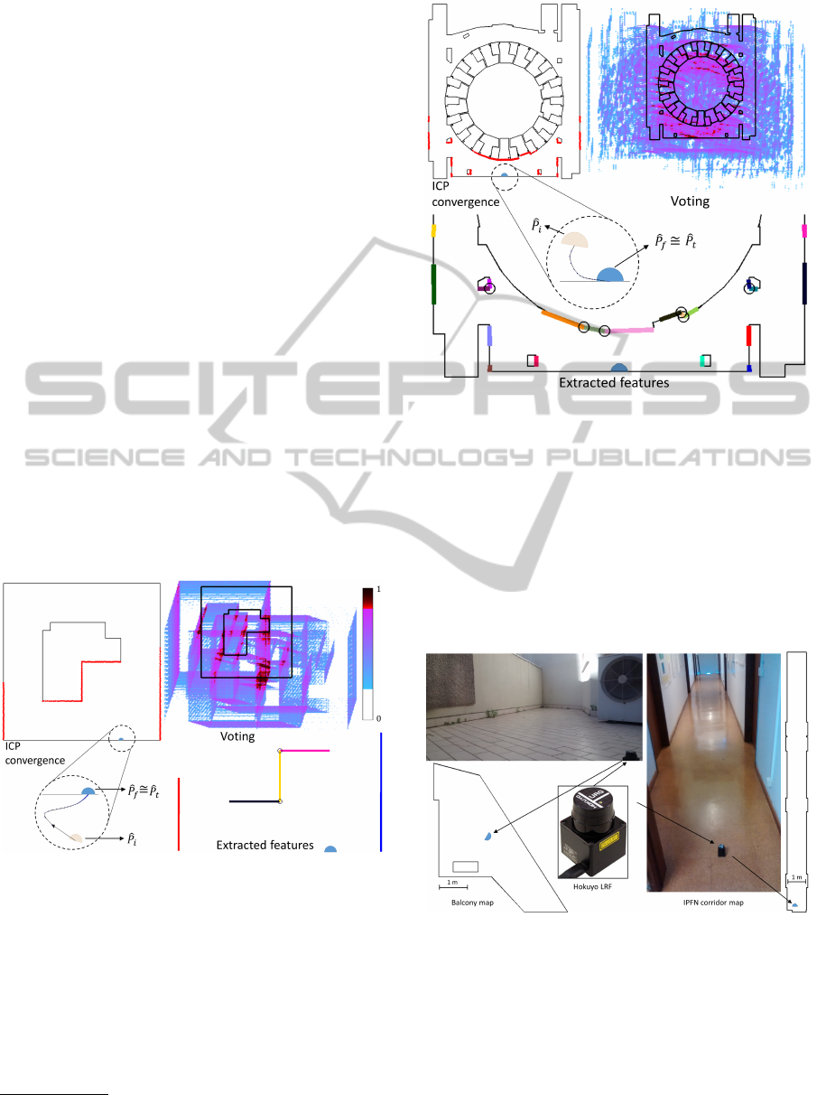
described in Section 3. Two maps, converted to points

with a density of 50 points per meter, with no outliers

in both, were used. The ﬁrst one is a simple created

asymmetrical map and the other a complex map from

ITER basement, where the actual CPRHS will navi-

gate, represented respectively from left to right in Fig-

ure 4.

Figure 4: LRF sensor used in simulation testing scenarios.

For each a model of a LRF was created featuring

the following main properties: 180

◦

of FOV, STD of

±50 mm, maximum range of 100 m, linear resolution

of 1 mm and angular resolution of 0.5

◦

. Each LRF

CalibrationofLaserRangeFindersforMobileRobotLocalizationinITER

545

were set in the predeﬁned poses represented in Figure

4, from where only one scan was taken. In scenario D,

the tolerance values that gave the best results, for the

clustering and feature extraction were the following:

0.5 m for proximity, 5

◦

for slope, 1 m for clustering

and 0.5 m for split.

The results obtained for the simple asymmetrical

map and for ITER map are presented in table 1.

in-

dicates the exact true pose where the measures were

taken from,

is an initial guess, at least, 1 meter

away from the true position,

is the ﬁnal pose re-

sulting from the algorithm output, “pp err.” is the

point to point error given by (1), “abs. error” is the

difference between true pose and ﬁnal pose and “RT”

(run time) is the time elapsed in the algorithm execu-

tion

. Images of the results are displayed respectively

in Figures 5 and 6. In each ﬁgure three images are

displayed: at the left side the ICP resultant alignment

of LRF points (in red) and the respective iterative evo-

lution from

, the heat map resulting from the

voting method is shown on the upper right section,

and on the lower section the geometrical features ex-

tracted (vertexes represented by the small circles) in

the vertex method are pictured. For scenario B an ar-

ray of 13 different and equally spaced angle values

were used and the result is not displayed because it is

similar to the ICP result.

Figure 5: Simulation results for asymmetrical map.

5 FIELD RESULTS

5.1 Sensors Speciﬁcation

The LRF device used was a Hokuyo URG-04LX-

UG01 (see Figure 7). The following main speciﬁca-

tions were taken from the respective device manual:

tests were always done on the same machine, an i5 proces-

sor.

Figure 6: Simulation results for ITER map.

240

◦

of FOV, STD of ±50 mm, maximum range of 4

m, linear resolution of 1 mm and angular resolution of

0.36

◦

. The LRF sensor was set in a predeﬁned mea-

sured position and orientation shown in Figure 7. At

least, data from one hundred scans were gathered and

processed to reject discrepant value measurements. In

scenario D, the tolerance values that gave the best re-

sults, for the clustering and feature extraction were

the following: 0.1 m for proximity, 15

◦

for slope, 0.1

m for clustering and 50 mm for split.

Figure 7: LRF sensor, photos and maps used in experimen-

tal testing.

5.2 Field Tests

Two distinct maps were used in the ﬁeld test as well,

one from a house balcony which contain some out-

liers, and the other from an ofﬁce corridor (Figure

7) composing a common environment of doors and

long walls. Both maps were converted to points with

ICINCO2015-12thInternationalConferenceonInformaticsinControl,AutomationandRobotics

546

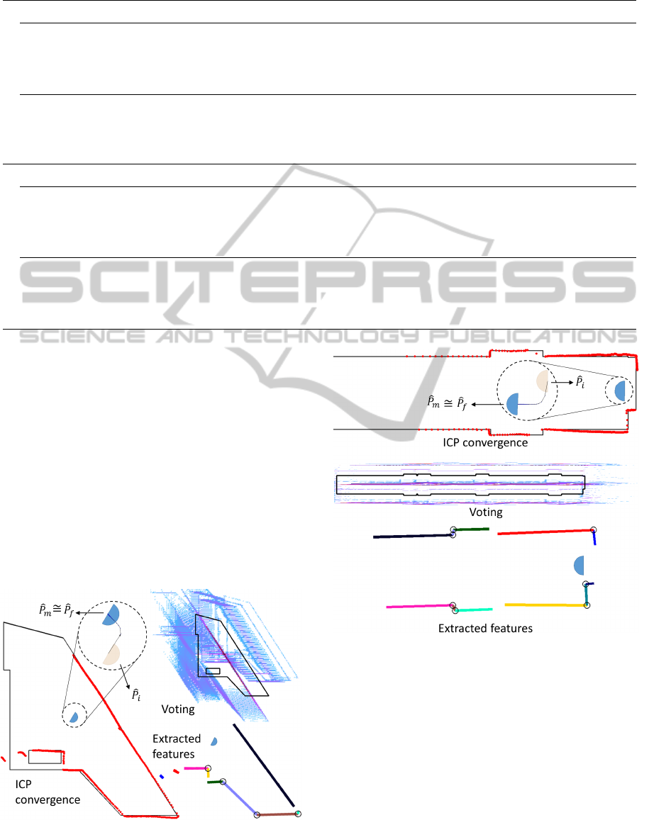
Table 1: Experimental results table.

Simulated Scenarios

Map Scen.

[m, m,

◦

]

[m, m,

◦

]

[m, m,

◦

] pp err. [mm] Abs. err. [mm,

◦

] RT[s]

Asymm.

(75.000, 0.000, 90.0)

(73.550,-5.280,73.0) (75.004, 0.002, 90.0) 53.1 (4.1, 0.0) 4.2

B (73.550, -5.280, -) (75.008, 0.007, 90.0) 53.1 (10.4, 0.0) 59

C (-, -, 73.0) (65.752, 0.852, 73.0) 4050.3 (9286.9, 17.0) 212

D (-, -, -) (75.013, 0.011, 90.0) 53.4 (17.4, 0.0) 5

ITER

(33.750, 1.000, 90.0)

(32.750, 2.000, 80.0) (33.750, 1.002, 89.9) 50.6 (2.0, 0.1) 4.3

B (32.750, 2.000, -) (33.750, 1.002, 89.9) 50.6 (2.0, 0.1) 48

C (-, -, 80.0) (27.303, 1.716, 80.0) 1928.5 (6487.0, 10.0) 1143

D (-, -, -) (33.713, 0.989, 90.0) 82.8 (38.5, 0.0) 33

Real Scenarios

Map Scen.

[m, m,

◦

]

[m, m,

◦

]

[m, m,

◦

] pp err. [mm] Rel. err. [mm,

◦

] RT[s]

Balcony

(1.700, 1.400, 330.0)

(1.700, 1.400, 330.0) (1.699, 1.452, 329.2) 44.6 (52.5, 0.8) 0.38

B (1.700, 1.400, -) (1.699, 1.452, 329.2) 44.6 (52.5, 0.8) 4.3

C (-, -, 330.0) (1.667, 1.457, 330.0) 79.6 (66.1, 0.0) 135

D (-, -, -) (1.599, 1.490, 330.7) 70.8 (64.3, 0.7) 1.4

IPFN

(14.750, 0.700, 180.0)

(14.750, 0.700, 180.0) (14.713, 0.665, 178.7) 26.3 (51.0, 1.3) 0.44

B (14.750, 0.700, -) (14.713, 0.665, 178.7) 26.3 (53.0, 1.3) 6.4

C (-, -, 180.0) (14.728, 0.707, 180.0) 41.6 (23.0, 0.0) 279

D (-, -, -) (14.720, 0.665, 178.7) 26.4 (46.7, 1.3) 7

a density of 50 points per meter except for the vot-

ing tests where the density was changed to 5 in or-

der to terminate the algorithm execution in a feasible

time. The results obtained for the balcony and corri-

dor maps are presented in table 1. The respective sec-

tion columns are identical to the columns of the sim-

ulated results explained before except for

which

means pose measurements, consisting the only way

to ﬁrst guess the initial pose (by hand measuring) so

a relative error column (“Rel. err”) was introduced.

Also images of the respective results are displayed in

Figures 8 and 9. The images follow the same layout

as the simulation ﬁgures stated above.

Figure 8: Balcony map experimental results.

Figure 9: IPFN map experimental results.

6 CONCLUSIONS

An algorithm to calibrate a LRF sensor network was

proposed. The outcome is an estimated pose for each

device in the network. Simulated and experimental

test results show a dependency of the pose estimate

error to the sensor and map description accuracy. The

developed algorithm receives three input parameters:

a map description of the environment, LRF data, and

an initial pose estimate for each device. The ﬁrst two

are mandatory and the uncertainty associated with the

CalibrationofLaserRangeFindersforMobileRobotLocalizationinITER

547

last one deﬁnes a scenario which determines the algo-

rithm behavior. Regardless of the scenario, the map

is always converted to points in order to assess the

results using (1). The map point conversion density

should be chosen accordingly as the previous equa-

tion presents an O(n

) operation.

Whenever an initial pose estimate is completely

known, the ICP algorithm is executed. The ﬁnal pose

estimate is revealed by applying the ICP resultant

rigid body transformation to the initial pose estimate.

This is the fastest and most accurate method but isn’t

robust against the presence of outliers in the LRF data

or map description. To reduce this negative effect, an

outlier rejection method is planned for future work.

An extreme scenario may occur when the pose

of the sensors is completely unknown. In this case,

ICP alone cannot be used because of its local min-

ima problem, therefore a developed vertex method is

applied. This method comprises two phases: ﬁrst,

geometric features, as segment lines and vertexes,

are extracted and subsequently a matching technique

based on the geometric combination of these features

is preformed. The main obstacle here is to ﬁgure out

the best combination of threshold values that leads

to a correct feature extraction. The time complexity

is proportional to the number of extracted features.

Other techniques, not as reliant on threshold values,

are on future plans. As an alternative, a brute force

test was conducted where the map was divided in a

grid and for each point of the grid, the ICP was ex-

ecuted. The results for the asymmetrical map are

shown in Figure 10. Although much more time con-

suming than the vertex method, slightly better accu-

rate results were achieved.

Figure 10: ICP brute force result.

As for the intermediate scenario, only the position

or orientation estimate value is known. In the ﬁrst

case, a brute force ICP is carried out in the given po-

sition for a set of predeﬁned angles. For the second

case, a voting based algorithm is applied to assign a

estimate probability of the LRF position to each of

the map coordinates. The voting method can be time

consuming and a less accurate method due to a combi-

nations of high initial angle deviation, low map reso-

lution and symmetry. Nevertheless suggests a consis-

tent alternative and a case of study for a global search

method.

An accurate map is assumed although, in a real

case scenario, that might not be the case. In the pres-

ence of outliers in the scanned data or map misde-

scription, robustness tests show that a variation of 1%

is enough to produce an error ten times higher. These

results, in the case of this application, can compro-

mise the localization algorithm behavior, where the

poses of the devices are to be used. In order to im-

prove outliers robustness, the ICP algorithm can be

customized to include an outliers rejection method.

ACKNOWLEDGEMENTS

The work leading to this publication received ﬁnan-

cial support from “Fundação para a Ciência e Tec-

nologia” through project UID/FIS/50010/2013. This

publication reﬂects the views only of the author, and

Fusion for Energy cannot be held responsible for any

use which may be made of the information contained

therein.

REFERENCES

A. Tesini, J. P. (2008). The iter remote maintenance system.

Fusion Eng. Des., 83(7-9):810–816.

Antone, M. and Friedman, Y. (2007). Fully automated laser

range calibration. In Proc. BMVC, pages 66.1–66.10.

doi:10.5244/C.21.66.

Besl, P. and McKay, N. (1992). A method for registration

two 3-d shapes. IEEE Trans. Pattern Anal. and Mach.

Intell., 14(2):239–256.

Carlos Fernández, Vidal Moreno, B. C. (2010). Cluster-

ing and line detection in laser range measurements.

Robotics and Autonomous Sys., 58(5):720–726.

Censi, A. (2008). An ICP variant using a point-to-line met-

ric. Robotics and Automation, pages 19–25.

Darren Locke, C. G. (2014). Progress in the conceptual de-

sign of the iter cask and plug remote handling system.

Fusion Eng. Des., 89(9-10):2419–2424.

J. Ferreira, A. Vale, R. V. (2013). Vehicle localization sys-

tem using off-board range sensor network. Proc. of

ICINCO2015-12thInternationalConferenceonInformaticsinControl,AutomationandRobotics

548

the 8th IFAC Intelligent Autonomous Vehicles Sympo-

sium, 8(1):102–107.

J. Soares, R. Ventura, A. V. (2014). Human-robot interface

architecture for a multi-purpose rescue vehicle for re-

mote assistance. In Symposium on Fusion Technology.

K. S. Arun, T. S. Huang, S. D. B. (1987). Least-squares

ﬁtting of two 3-d point sets. Pattern Analysis and Ma-

chine Intelligence, IEEE Transactions, 9(5):698–700.

K. Schenk, A. K. (2012). Automatic calibration of a station-

ary network of laser range ﬁnders by matching move-

ment trajectories. IEEE/RSJ Int. Conf. on Intelligent

Robots and Systems, pages 431–437.

Low, K.-L. (2004). Linear least-squares optimization for

point-to-plane ICP surface registration. Tech. report.

Markus-Christian Amann, Thierry Bosch, M. L. R. M.

M. R. (2000). Laser ranging: a critical review of

usual techniques for distance measurement. Opt. Eng.,

40(1):10–19.

Sebastian Thrun, J. L. (2008). Handbook of Robotics.

Springer.

Viet Nguyen, Stefan Gächter, A. M. N. T. R. S. (2007).

A comparison of line extraction algorithms using 2d

range data for indoor mobile robotics. Autonomous

Robots, 23(2):97–111.

Vincenzo Caglioti, Alessandro Giusti, D. M. (2008). Mu-

tual calibration of a camera and a laser rangeﬁnder.

Proc. Int’l Conf. on Computer Vision Theory and Ap-

plications, pages 33–42.

CalibrationofLaserRangeFindersforMobileRobotLocalizationinITER

549