
A Formation Control Algorithm by Modified Next-state
Approximation to Reduce Communication Requirements in
Multirobot Systems
Roshin Jacob Johnson
1
and Asokan Thondiyath
2
1
Department of Mechanical Engineering, Indian Institute of Technology Madras, Chennai, India
2
Department of Engineering Design, Indian Institute of Technology Madras, Chennai, India
Keywords: Formation Control, Multi Robot System, State Estimation, Leader-follower Control, Underwater Robots,
AUV.
Abstract: Multiple robot systems are employed in various applications to get the complex tasks carried out by a group
of robots. When Autonomous Underwater Vehicles (AUVs) are employed for underwater missions, they
provide higher quality data, more coverage and reduces the mission time, thus resulting in huge cost savings.
However, the formation control of such robots depends to a great extent on the communication requirements
between the robots. In this paper, we propose a modified next-state approximation algorithm to control the
leader follower formation of multiple AUV’s which reduces the communication requirements. The controller
drives each follower robot to the next desired position by eliminating the error between the next actual position
of follower AUV, computed by considering its current and previous position and its next desired position by
using a PID controller. Since this algorithm is independent of time step between states, the amount of
information to be transmitted can be reduced by increasing the time steps. The design of the formation
controller and its simulation studies for a group of AUVs are presented. The results confirm that the time step
increase doesn’t affect the path accuracy and hence the communication requirements get reduced.
1 INTRODUCTION
Multiple robots are used to perform various tasks in
an efficient way. Multiple AUVs are increasingly
being considered as a means to perform research,
survey and defense missions in underwater. Their
formation control has become an area that has evoked
the attention of several researchers in recent times.
Currently, there are three main approaches for
formation control, namely, behavior based method
(Balch and Arkin, 1998), virtual structure method
(Ren and Beard, 2003), and leader follower method
(Chen and Serrani, 2003). In behavior based approach
several behaviors are taken into account and action is
taken by weighing the relative importance of each
behavior. The main problem of this approach is the
difficulty in mathematical formalization and as a
result convergence of formation to desired
configuration cannot be easily guaranteed. The virtual
structure approach considers the formation as a single
virtual rigid structure. The difficulty with this
approach is that a large inter robot communication
bandwidth is required. In leader follower approach an
AUV is assigned as leader and others as followers.
The followers are supposed to maintain a desired
distance and orientation with respect to the leader
AUV, thereby forming a formation as a whole. The
reference trajectory and the missions for the entire
trajectory will be communicated only to the leader
AUV. Thus there will be only local communication
between leader and follower rather than global,
thereby ensuring flexibility and mission safety.
Many of the existing formation controllers try to
sense the current position of follower AUV and align
it to desired path. This may result in slow response,
and convergence to desired trajectory can be
troublesome when there is an unexpected change in
leader trajectory. In one of the earlier works, a state
estimation algorithm was proposed where the
follower AUV tries to estimate its future position and
operating scenarios and drives itself to the desired
future state (Neettiyath and Thondiyath, 2012). This
method is advantageous when compared to other
leader follower methods as it focuses on eliminating
275
Jacob Johnson R. and Thondiyath A..
A Formation Control Algorithm by Modified Next-state Approximation to Reduce Communication Requirements in Multirobot Systems.
DOI: 10.5220/0005537502750280
In Proceedings of the 12th International Conference on Informatics in Control, Automation and Robotics (ICINCO-2015), pages 275-280
ISBN: 978-989-758-123-6
Copyright
c
2015 SCITEPRESS (Science and Technology Publications, Lda.)
the error at the next position rather than at the current
position. As a result of this, the response time
decreases and alignment with desired path takes place
quicker. However, the next-state estimation depends
on the time-step and as the time step increases the
path error increases. This necessitates very small
time-steps to reduce error and it leads to increased
communication between leader and follower. This is
not at all desirable as underwater communication is
generally slow and noisy.
In this paper we present an algorithm which is an
improved version of state estimation based formation
control algorithm presented in (Neettiyath and
Thondiyath, 2012). Changes are brought about in the
way the next state is estimated and also on how the
error between the next estimated and desired position
is reduced. The next position was computed by
considering a general path for the motion of AUVs
and stability was maintained by removing the error
between the next desired position and estimated
position by adapting and modifying the error removal
method mentioned in (Consolini et al., 2008). This
method reduces the communication among AUVs as
the number of pose calculations are reduced. The
paper is organized in the following way: Section 2
describes the algorithm in detail. The method of
implementation and results are discussed in section 3.
Section 4 summarizes the paper and indicates the
scope and future work.
2 FORMATION CONTROL
ALGORITHM
In Section 2.1 method of next state approximation for
a leader-follower type formation control is explained
and in section 2.2 method of stabilization by error
removal is explained.
2.1 Next-state Estimation
According to (Neettiyath and Thondiyath, 2012), the
next state is estimated as follows:
η
Le
(t+1) = η
L
(t) + ( η
L
(t) - η
L
(t-1) )
(1)
η
Fe
(t+1) = η
F
(t) + ( η
F
(t) - η
F
(t-1) ) (2)
where η
F
and η
L
represents pose (x, y, z, Roll (φ),
Pitch (Θ) and Yaw (ψ) - Here 2 dimensional case is
being considered, therefore z, Roll (φ) and Pitch (Θ)
do not change and are taken to be equal to zero) of the
follower and leader respectively and η
Fe
and η
Le
represents the estimated position of the follower and
leader AUV and this is calculated for time t+1(next
position).
This is done on the assumption that the AUV
undergoes uniform motion. For any general case the
above equation is valid for Yaw (ψ) - Angular
orientation at next position is equal to current plus the
change between the current and the previous. But
when this is done for both x and y coordinate the next
position will lie on the straight line joining current
and previous position. This means by default it is
assumed that the trajectory is straight line, which is
not true.
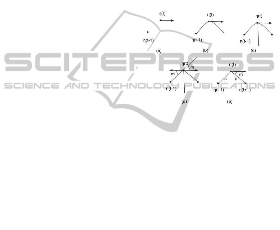
Figure 1: Next state estimation.
The next position (η
(t+1)) should lie on an arc
connecting previous (η
(t-1)) and current position (η
(t)), with the current orientation being tangent to the
arc (Figure 1-(b)). By assuming uniform motion the
next and previous positions (x, y) should be
symmetric with respect to the normal to current
orientation (Figure 1-(c)). The distance between the
current and previous position should be same as that
between the next and current position. Let ‘m’ be the
angle the line joining current position with previous
position makes with the negative of current
orientation which is same as the angle that the line
joining previous to current position makes with
current orientation (Figure 1-(d)).
mtan
ψ
(3)
where x(t) and y(t) are x and y coordinates at time t.
Symmetry condition shows that the angle between
current orientation and the line joining current to next
position should also be m (Figure 1-(e)).
Therefore final position is given by
η[1] = x(t+1) =x(t) + s * cos(ψ(t) - m)
(4)
η[2] = y(t+1)= y(t) + s * sin(ψ(t) - m) (5)
where
s= ((y (t)-y (t-1))
2
+(x (t)-x (t-1))
2
)
0.5
(6)
ICINCO2015-12thInternationalConferenceonInformaticsinControl,AutomationandRobotics
276
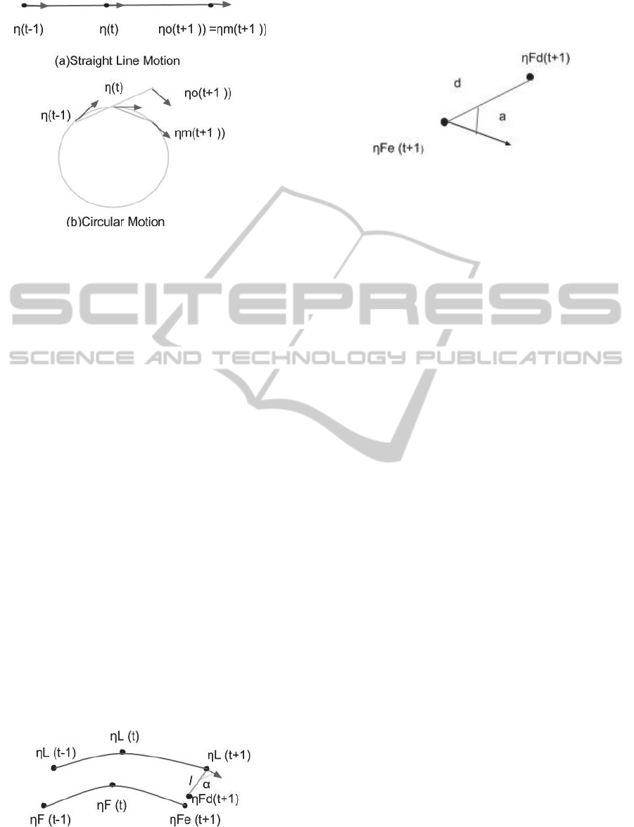
Figure 2: Comparison of Next state estimated by two
methods.
The next position calculated by the method
mentioned in (Neettiyath and Thondiyath, 2012)
(η
o
(t+1 )) and the above mentioned modified method
(η
m
(t+1 )) for two different cases of motion (straight
line and circular ) is shown in figure 2. It is clear from
the figure that for straight line motion estimated
position by both methods remains same but for
circular motion it is evident that the modified method
gives correct solution. Therefore we can conclude
that the modified next state estimation method is
better for a general case.
The next positions of leader and follower was
calculated by above method. In the case of L- α
method of formation control (Neettiyath and
Thondiyath, 2012), the desired next position of the
follower can be computed from expected next
position of leader and from l and α values using pure
geometry as
η
Fd
(t+1)=η
Le
(t)+R(ψ(t+1)) R(α)
0
(7)
Where R ( ψ(t+1)) is rotational matrix and ψ(t+1) is
the yaw angle of leader at ‘t+1’.
R (x) =
cos sin 0
sin cos 0
001
(8)
Figure 3: Position of leader and follower at different time.
2.2 Stabilization Making the Error
Zero
Figure 4: Estimated and desired position of follower.
As shown in figure 4 let 'd' denote the distance
between the desired follower position and estimated
actual follower position at time 't+1'.Let 'a' denote the
angle this line makes with the orientation of the
follower AUV. Then
δv = d * cos(a)
(9)
δω = d * sin(a) (10)
Where δv and δω represents the linear and angular
velocity error respectively.
This error was given as an input to the PID
controller which finally reduces it to zero. Linear and
Angular velocity at time t+1 can be written in terms
of the current velocity and this error.
v(t+1)=v(t)+K
pv
(δv)+K
iv
Σ( δv )+K
dv
( Δ(δv)
(11)
ω(t+1) =ω(t)+K
pω
(δω)+K
iω
Σ(δω)+ K
dω
(Δ(δω)
(12)
Several tuning methods are there to obtain
Proportional Gain (K
p
), Integral Gain (K
i
) and
Derivative Gain (K
d
) where subscript v and ω indicate
that it corresponds to linear and angular velocity
respectively. Manual tuning was used in our
experiment. The major advantage of stabilization by
this method over that in (Neettiyath and Thondiyath,
2012) is that it does not depend upon time step
between different states.
3 IMPLEMENTATION AND
RESULTS
The proposed algorithm was developed and tested
using simulation by modeling the system in
Matlab/Simulink. Dynamics was taken into account
while modeling the AUV. In the following sections
the implementation method and few of the
simulations implemented are explained.
3.1 Implementation
Figure 5 shows the formation controller
AFormationControlAlgorithmbyModifiedNext-stateApproximationtoReduceCommunicationRequirementsin
MultirobotSystems
277
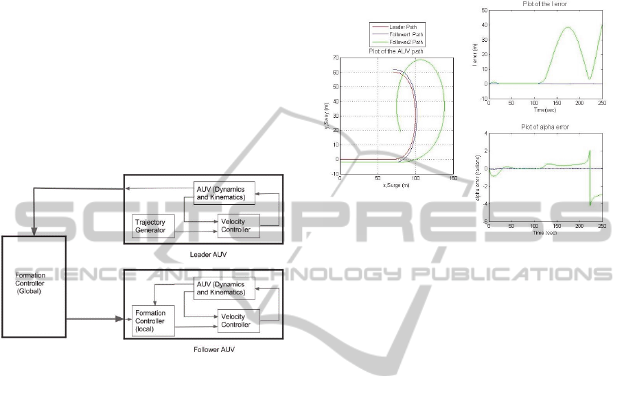
implementation for the leader follower formation.
Formation controller (Global) is used to supply the
formation parameters to the individual followers at
each point of time, thereby holding the formation
together. The parameters can be changed with respect
to time to obtain different formations. The leader
AUV has 'Trajectory Generator' block which
generates the trajectory of motion, whereas follower
AUV has Formation Controller (local) which uses the
proposed algorithm to compute the velocity
correction signal. AUV is maintained at a specified
velocity by actuating the thrusters in the velocity
controller. Kinematics and Dynamics of the AUV
was modeled and incorporated as in (Neettiyath and
Thondiyath, 2012; (Fossen, 1994); (Yuh, 2000).
Figure 5: Formation controller implementation.
3.2 Results
3.2.1 Comparison
A situation was considered when the leader initially
moved in a straight line path and then in a
semicircular arc (Figure 6-(a)). Two followers were
made to follow the leader in same paths maintaining
a constant formation [l=2 α = -90
0
]. Follower 1 uses
the proposed strategy whereas follower 2 uses the old
one. Both follows the leader in the desired path when
the leader underwent straight line motion. But when
leader started moving in the semicircular arc follower
1 moved in the desired path whereas follower 2
started deviating from the path and finally ended up
losing track. Follower 1 maintains the formation till
the end with minimal error (l and α) (Figure-6 (b),
(c)).
Even Follower 2 will maintain the desired path if
the time step is decreased. But this means that an
increase in the total number of computations. The
effect is clearer when the time step increases
exponentially. Initially time step [t
0
] is considered
such that follower 2 follows the leader (Figure 7-
(a)).Then time step is made 10t
0
(Figure 7-(b)) and
100t
0
(Figure 7-(c)) during which follower 2 loses
track when leader starts moving in circular part. In all
three cases follower 1 moves in the desired path with
minimum error.
Figure 6: Comparison of both Algorithms under constant
formation.
This result has large implications as the number of
computations of the next state can be brought down
by increasing time steps. This means that the number
of times the follower communicates with the leader
can be brought down which is highly desirable in
underwater systems where communication occurs
slowly and in a noisy environment.
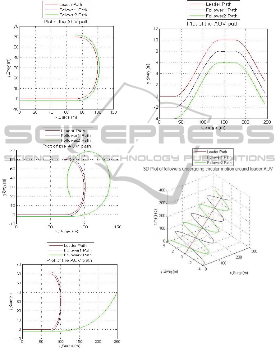
3.2.2 Constant Formation
The position of each follower AUV in the formation
with respect to the leader AUV was maintained
constant. In Figure 8 leader was made to move
horizontally initially, then in an upward inclined path
followed by horizontal path and finally a path that is
inclined downwards. Both followers were maintained
at α = -90
0
and l value was 2 and 4 respectively for 1
and 2. It is seen that the follower maintains the
formation.
3.2.3 Variable Formation
Simulation was done for the case when formation
varies with respect to the leader. A situation was
considered when the leader moves in a straight line
and the followers undergoes circular motion around
the leader. The radius of rotation changes from 4 (l=4)
to 2 (l=2) for both followers at the same time α
changes from -90
0
to 990
0
for the first follower
whereas it changes from 90
0
to 1170
0
for the second.
Each follower completes 3 rotations around the leader
AUV. A 3D plot of the same is shown in figure 9.
ICINCO2015-12thInternationalConferenceonInformaticsinControl,AutomationandRobotics
278
(a)
(b)
(c)
Figure 7: Comparison of motion for different time steps.
Figure 8: AUV Motion when the formation is fixed.
Figure 9: 3D plot when followers undergoes a circular
motion around leader.
4 CONCLUSIONS
An improved state estimation algorithm is proposed
and simulations have been done to prove its validity.
The main advantage of this algorithm over the already
existing one is that the communication between
leader and follower AUVs can be brought down,
which is a highly beneficial result as underwater
communications are generally slow and noisy. This
also results in reduction in the number of
computations and the dependency on time step
AFormationControlAlgorithmbyModifiedNext-stateApproximationtoReduceCommunicationRequirementsin
MultirobotSystems
279

between states has been eliminated. This algorithm is
mainly applicable in situations where the number
sudden changes in direction of motion is low in the
entire path of motion. Future work would be to extent
this algorithm to 3 Dimensional motion of robots.
ACKNOWLEDGEMENTS
I wish to express my sincere thanks to Umesh
Neettiyath, Research Scholar, for extending his
invaluable help and support in making the simulation
model to test the proposed algorithm.
REFERENCES
T. Balch, R. C. Arkin, "Behavior-based formation control
for multirobot teams”. IEEE Transaction on Robotics
and Automation, 1998. 14(6).pp.926-939.
W. Ren, R. W. Beard, “A decentralized scheme for
spacecraft formation flying via virtual structure
approach”. Proceedings of the American Control
Conference Denver, Colorado, American Automatic
Control Council 2003, pp.1746-1751.
X. P. Chen, A.Serrani, H.Ozbay, “Control of leader-
follower formations of terrestrial UAVs”. IEEE
Conference on Decision and Control, Hawaii: IEEE,
2003. pp.498 – 503.
U. Neettiyath and A. Thondiyath. “Improved leader
follower formation control of autonomous underwater
Vehicles using state estimation”. In Proceedings of the
9th International Conference on Informatics in Control,
Automation and Robotics, pages 472{475.SciTePress -
Science and Technology Publications, 2012.
L. Consolini, F. Morbidi, D. Prattichizzo, and M. Tosques.”
Leader-Follower Formation Control of nonholonimic
mobile robots with input constraints”. Automatica,
44(5):1343-1349, 2008.
G. Antonelli, T. I. Fossen, and D. R. Yoerger.Underwater
robotics. In B. Siciliano and O. Khatib, editors,
“Springer Handbook of Robotics”, chapter 44, pages
987{1008. Springer Berlin Heidelberg, Berlin,
Heidelberg, 2008.
T. I. Fossen. “Guidance and control of ocean
vehicles.”Wiley, 1994.
J. Yuh. “Design and control of autonomous underwater,
robots: A survey”. Autonomous Robots, IEEE
conference, San Francisco 8(1):7{24, Jan.2000.
ICINCO2015-12thInternationalConferenceonInformaticsinControl,AutomationandRobotics
280
