
The Impact of Household Structures on Pandemic Influenza Vaccination
Priority
Hung-Jui Chang
1,2
, Jen-Hsiang Chuang
3
, Yang-Chih Fu
4
, Tsan-Sheng Hsu
1
, Chi-Wen Hsueh
2
,
Shu-Chen Tsai
1
and Da-Wei Wang
1
1
Institute of Information Science, Academia Sinica, Taipei, Taiwan
2
Depart of Computer Science and Information Engineering, National Taiwan University, Taipei, Taiwan
3
Epidemic Intelligence Center, Centers for Disease Control, Taipei, Taiwan
4
Institute of Information Social, Academia Sinica, Taipei, Taiwan
Keywords:
Household Structure Distribution, Agent-based Simulation, Vaccination Policy.
Abstract:
The household structure is an important aspect of population based simulation. How to generate a mock pop-
ulation with specific household structure characteristics is thus an important question. The network structure
is one of the dominant factors for contact-based disease transmission. And household structure is the most
important source of close contact among small groups. We identify the percentage of elderly-children house-
holds as an important character and study the process to generate mock population with specified percentage of
elderly-children households. The generated mock populations are fed into the agent-based simulation module
to study the impact of household structure on vaccination policy.
1 INTRODUCTION
Household structures are important for many appli-
cation domains. Household structures change over
time and vary geographically and culturally (OECD,
2011). Network structures affect the disease spread-
ing patterns. Household structure is an important
component of the transmission network of infectious
disease. Because of the strong interactions present,
households are one of the most important hetero-
geneities to consider, both in terms of predicting epi-
demic severity and as a target for intervention (House
and Keeling, 2009).
Family are different in different area. Among
the Asian countries, at least 80 percent of children
are raised by two-parent families, and at least 40
percent are also living with extended family mem-
bers (Trends, 2013), while in Europe at least 15
percent are living with extended family members.
For example, the percentage of households where
grandparents live with grandchildren is reported to be
ranged from 9.2 percentage to 20.5 percent in Asia
and from 0.1 percent to 3.9 percent in western and
northern Europe, Table 1.
Taiwan is approaching an aging society at an
Table 1: The household structure in Europe and
Asia(http://ec.europa.eu/).
country m<15 & M≥65(%)
Asia
Indonesia <09.2
Taiwan <15.0
Thailand <16.5
Vietnam <20.5
Europe
Belgium <00.1
Finland <00.9
Germany <01.1
Italy <03.1
Luxembourg <00.7
Netherlands <00.1
Poland <03.9
United Kingdom <00.9
M: the oldest person’s age in a family.
m: the youngest person’s age in a family.
alarming rate, due to the rapid decline of birthrate as
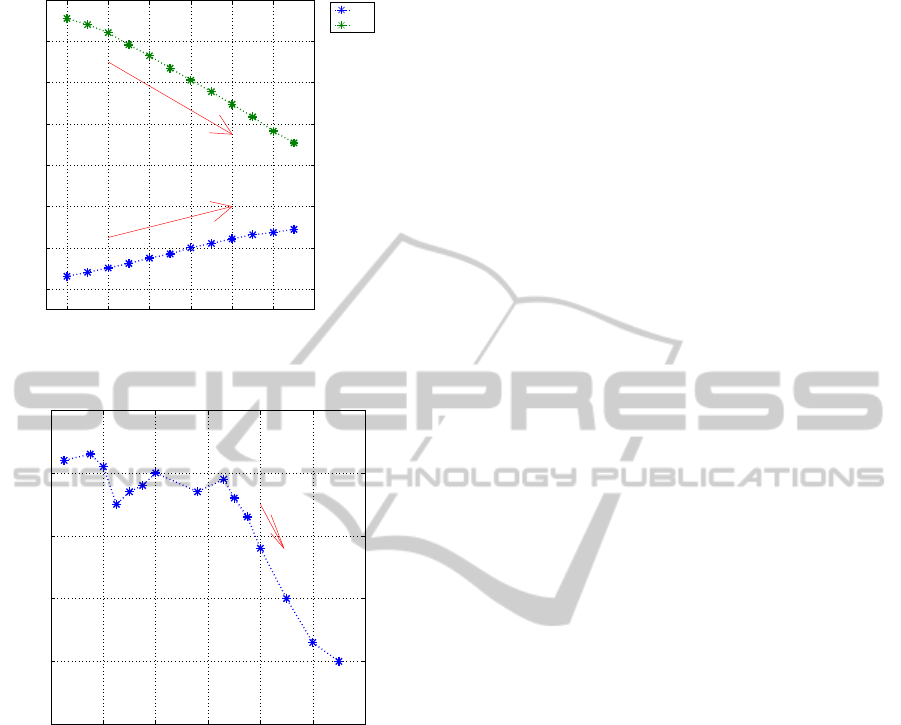
well as longer life expectancy. As shown in Figure
1, from 2000 to 2012, the youth population (less then
15 years old) dropped from 21 percent to 15 percent,
while senior population (age 65 and up) increased
from 8 percent to 11 percent. The average household
size is also declining for decades, from 5.9 in 1966
to 3.0 in the 2010, Fig 2. It is conceivable that the
482
Chang H., Chuang J., Fu Y., Hsu T., Hsueh C., Tsai S. and Wang D..
The Impact of Household Structures on Pandemic Influenza Vaccination Priority.
DOI: 10.5220/0005539204820487
In Proceedings of the 5th International Conference on Simulation and Modeling Methodologies, Technologies and Applications (SIMULTECH-2015),
pages 482-487
ISBN: 978-989-758-120-5
Copyright
c
2015 SCITEPRESS (Science and Technology Publications, Lda.)
2000 2002 2004 2006 2008 2010 2012
8
10
12
14
16
18
20
22
Ratio(%)
The ratio of 65+ and 0-14 in Taiwan
65+
0-14
Figure 1: The ratio of over 65 years old and 0-14 in
Taiwan(2000–2011).
1900 1920 1940 1960 1980 2000 2020
2
3
4
5
6
7
Household Size
The Household Size in Taiwan
Figure 2: The household size in Taiwan(1900–2010).
living or parenting arrangements in Asia may differ
from those in the West. It is not uncommon in Tai-
wan that grandparents live with grandchildren, or for
grandparents to help taking care of their young grand-
children on a daily basis. In such a circumstance,
both care givers (seniors) and care takers (toddlers or
young children) may have much more contact than
their counter parts in countries where seniors do not
live with young children. And the fact that these two
age groups are also most susceptible to influenza in-
fections makes this pattern evenmore interesting from
disease prevention perspective. ”Does this special
feature of age composition within the household con-
tribute to any divergent cross-cultural patterns of dis-
ease infections? When contact patterns in everyday
life are subject to such cultural norms, policy makers
should make the best use of diary-generated empirical
data and design intervention strategies accordingly”
(Fu et al., 2012).
We study the household structure of two cen-
sus data from Census 2000 and Census 2010 in Tai-
wan. In order to study the impact of household struc-
ture on epidemiology, we have to find a method to
generate mock population with specific household
structure characteristics. A simulation approach to
generate household structure is proposed by Geard
et al. (Geard et al., 2013). In this paper we pro-
posed to formulate it as a mathematical program-
ming. The specific household characteristics are the
primary constraints and other ”desired properties” are
secondary constraints. The generated mock popula-
tions are applied to explore the impact of household
structure on vaccination priority for influenza. We
use the agent-based disease spreading simulation soft-
ware to carry out our studies (Tsai et al., 2010). The
concepts of the simulation software is similer to Ger-
mann’s work.(Germann et al., 2006). And based on
the census data from 2000 and 2010 to generate our
initial sample population. Given a specified ratio of
elderly-children households, a transformation process
is developed to generate the sample population with
the given ratio from the initial population. Two vac-
cination policies are compared, namely, school chil-
dren only and elderly only. The rationales to vaccine
school children only are two folds. First, students
have close contact with each other, vaccinating stu-
dents can reduce the number of students infected by
other students. So that the chance of a school age
kid brings virus home is reduced. Second, it is more
cost effective to vaccinate students because they are
at a centralized location - the school. The rationale to
vaccinate elderly only is mainly to reduce the number
of severe cases and fatal cases.
We note that the selected vaccination policies are
only for demonstration the effect of household struc-
ture on disease spreading.
2 MATERIAL AND METHOD
The household structure for the generation of a mock
population is a probability distribution over house-
hold patterns.
The specific of the possible patterns depends on
the applications. In this paper, the entire population
is classified into five age groups: preschoolers (0−4
years old), school-age children (5−18 years old),
young adults (19−29 years old), adults (30−64 years
old), and elders (65+ years old). And a household
pattern is a ten dimensional tuple, for 5 age groups
and genders, that is we keep track on the number
of males and females in each age group of a house-
hold. We set seven to be the upper bound of each
TheImpactofHouseholdStructuresonPandemicInfluenzaVaccinationPriority
483

entry. Therefore, there are 8
10
possible patterns and
each pattern can be encoded in 4 bytes. Let H denote
the set of patterns, a household structure distribu-
tion(HSD) is a probability space, (H, p) where func-
tion p maps an element in H to a probability. A char-
acteristic of household structure is a measurement of
the HSD. For example, the percentage of elders (over
65), or the percentage of households with preschool-
ers and elders. However, it would be difficult to know
the percentage of household in which children live
with both parents because we do not capture that rela-
tion in our setting. Usually, we have some other data
related to or constraint on household structure distri-
bution such as the age distribution of the population.
In general, we can treat any statistical measurements
of a population as soft constraints and the goal is to
generate a mock population that ”satisfies” them.
Since all the surveys and measurements are snap-
shots and subjected to noises, it is usually impossible
to satisfy all the constraints. For our study, the impor-
tant characteristic of a HSD is the elder-children ratio
(EC ratio), which is the percentage of householdswith
elderly and a young person under 15. Since the HSD
does not capture enough information to determine if
a school-age child is under or over 15 years old, we
have to utilize the age distribution data from the cen-
sus to decide stochastically the age of a school-age
child.
The mock population is constructed according to
national demographics and daily commuter (worker
flow) statistics from Taiwan Census 2010 Data
(http://www.stat.gov.tw/) in order to retain some pop-
ulation characteristics.
The generated mock population with desired HSD
is fed into the simulation software developed by Tsai
et al. (Tsai et al., 2010). Below is a brief description
of the simulation module.
The connection between any two individuals indi-
cates the possibility of regular (daily) and relatively
close contact that could result in the successful trans-
mission of the flu virus. An important parameter is the
disease depends on transmission probability denoted
P
trans
. It is the probability that an effective contact
results in an infection.
A contact group is a close association of individ-
uals, where every member is connected to all other
members in the group. We designate ten classes of
such contact groups in our model: community, neigh-
borhood, household cluster, household, work group,
high school, middle school, elementary school, day-
care center, and playgroup. It is important to note that
these contact groups do not represent all people at any
physical location such as a workplace or school, but
rather the groups of people who share the same sur-
rounding activities and sustain regular close contact
for potential viral infection.
Each individual is a member of one of the five age
groups throughout the simulation can belong to sev-
eral contact groups simultaneously at any time. The
probability of any two individuals staying in contact
that could result in the successful transmission of the
flu virus is called the contact probability, and an em-
piric value is assigned depending on the group where
contact occurs and the ages of both individuals.
Age not only affects the probability of an individ-
ual being infected, it also determines the individual’s
daytime contact groups: preschoolers stay either in
daycare centers or in playgroups; school-age children
stay either in schools or in households as dropouts;
young adults and adults stay either in work groups or
in households if unemployed.
Each simulation runs in cycles of two 12-hour pe-
riods, daytime and nighttime, with each cycle repre-
senting a day in the simulation. The simulation can
cover any specified duration of days; we usually oper-
ate in 180 days for typical influenza season, but there
are times when 365 days duration is imperative for a
slow progressing epidemic. Contact occurs between
individuals in each contact group every day, there are
no exceptions for weekends or holidays until we can
properly ascertain their effects.
During nighttime, contact occurs only in commu-
nities, neighborhoods, household clusters, and house-
holds; whereas in the daytime, contact occurs in all
contact groups. Children do not go outside of their
residential community for daytime activities because
the probabilities for such occasional contacts are too
low to be captured by any contact group. The only
inter-community transmission occurs when working
adults commute between household and work group
as specified by worker flow data as well as school
children commute between household and school as
specified by school flow (Tsai et al., 2010).
To derive a series of household structure with
specified EC ratio, we designed a simple household
structure evolution process to transform the set of pa-
rameters so that the percentageof EC household in the
mock population generated by the modified parame-
ters is sufficiently close to the designated number. We
formulate the process as a linear programming prob-
lem, the objective function is designed to avoid intro-
ducing dramatic ”changes” to other important aspects
of the household structures. The detail is described in
Figure 3.
A simulation setting is a set of parameters, which
include p
trans
and household structure. To study the
effect of vaccine policies, we fix a simulation setting
and simulate each vaccination policy. For each policy,
SIMULTECH2015-5thInternationalConferenceonSimulationandModelingMethodologies,Technologiesand
Applications
484
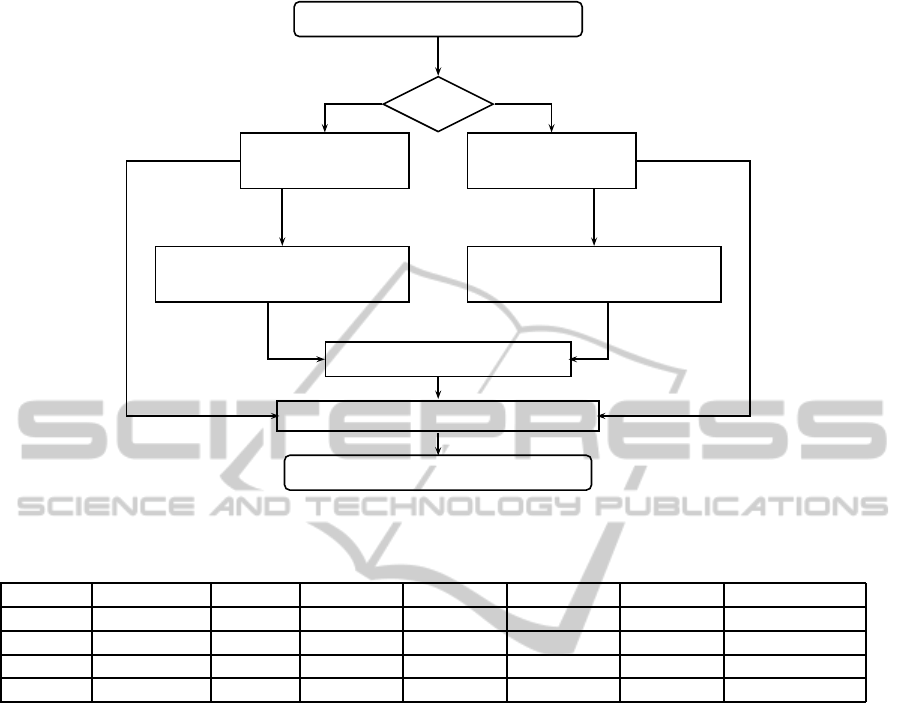
Input Household Structure
Is EC?
Yes No
EC family Non-EC family
Calculate Modification
Bounded Condition Constraint condition
Linear Programmming
Combine Household Structure
Turned size
Original size
Output Household Structure
Figure 3: Flow Chart of Using Linear Programming.
Table 2: The household size in each EC ratio(mock population).
EC ratio #population #0-4 #5-18 #19-29 #30-64 #65+ household size
30% 23,088,322 972,361 4,265,569 3,079,993 11,588,807 3,181,592 3.09
20% 23,087,718 938,074 4,217,799 3,124,340 11,686,059 3,121,446 3.05
10% 23,086,465 897,650 4,156,653 3,182,322 11,791,448 3,058,392 3.01
0.0% 23,079,732 970,817 4,262,075 3,078,738 11,590,107 3,177,995 2.78
’#’: the number of
we first carry out the baseline simulation which is the
simulation without any intervention. Then the simu-
lation with intervention policies are carried out with
the same setting. We start the vaccination at the 70
th
days and the number of available vaccine is 1.8 mil-
lion doses, the vaccine efficacy is set at 36%− 90%.
For each simulation run, we record the number of
infected cases for each group. We then take the aver-
age of simulation runs with the same setting and in-
tervention policy to be the outcome of that specific
policy.
The difference between the baseline and a inter-
vention policy is the effect of the intervention, and in
our case it is the difference of the number of infected
cases of each age group.
Note that we compare different policies with the
same setting and only focus on the number of infected
cases for each age group. If the numbers of reduced
infected cases for one policy, A, is always better than
the other policy, B, we can safely conclude that policy
A is superior than policy B. However, if a vaccination
policy is to set the priority of receiving vaccination
among age groups, it will be difficult to find a supe-
rior policy because a policy targeted at a specific age
group always results in the fewest infected cases for
that group.
We introduce a cost function, C which maps a five
dimensional point (the numbers of infected cases for
each age group) to a real number. Given a policy A,
the cost saved by A is C(base) −C(A), that is the cost
difference between baseline and policy A. We say that
policy A is better than policy B with respect to cost
functionC, if and only if the cost saved by A is greater
than B. For example, if we define C(n
1
, n
2
, n
3
, n
4
, n
5
)
to be the summation of the five numbers, we are com-
paring the number of infected cased reduced. The
costs of infected cases among different age groups
can be different (Meltzer et al., 1999). Here we adopt
a cost function which highlight the different between
elderly and others. Let C be a cost function with pa-
rameter α be:
C
α
(n
1
, n
2
, n
3
, n
4
, n
5
) = n
1
+ n
2
+ n
3
+ n
4
+ α∗ n
5
Function above captures the idea that the cost of
an elderly case is α times of the other age groups and
TheImpactofHouseholdStructuresonPandemicInfluenzaVaccinationPriority
485

the costs of all the other age groups are the same. We
define an equilibrium point for policy A and B to be
α∗ such that C
α∗
(A) = C
α∗
(B). Since C
α
is a linear
function, there is a unique equilibrium point between
two policies.
3 RESULTS
From the HSD perspective, the census data from
2000(C2000) and 2010(C2010) can be described as
following: there are 11283 household patterns in
C2000, 7072 in C2010 and a total of 11543 patterns
ever appeared in C2000 or C2010. There are 6813
patterns appeared in both C2000 and C2010. The
summation of the probability of the common pat-
terns is greater than 0.99 for both C2000 and C2010.
The Pearson correlation between these two HSDs is
around 0.95. There are 4470 patterns only appeared
in C2000 while 259 only in C2010. The apparent dis-
crepancy is due to the fact that C2010 only survey 16
percent of the household while C2000 surveyed every
household.
Based on processes described above, we success-
fully generated populations with specified character-
istics. In Table 2, the generated mock populations
have specified EC ratio, and the population is highly
correlated with original population, the Pearson cor-
relation ranging from 0.998 to 0.999.
The R
0
for the baseline case of each mock popu-
lation is calculated and summarized in Table 3. We
note that with the same transmission probability, the
lower the EC ratio the smaller the R
0
. And this can
be explained by the fact that average household size
decreases as EC ratio decreases. That is the differ-
ence of the network structure is the main reason for
the variation in the table.
We compare two vaccination policies, student
only and elder only. The results are summarized in
Table 4.
From the summary, we note that the student only
policy outperforms elder only for all age group except
seniors. That is the student only policy reduced the
number of infected cases more than elder only policy
in all four age groups excluding seniors. The can be
Table 3: R
0
.
transmission probability
EC ratio 0.08 0.09 0.10 0.11
30% 1.055 1.194 1.308 1.442
20% 1.053 1.182 1.302 1.432
10% 1.041 1.169 1.294 1.428
0.0% 0.910 1.122 1.247 1.352
50 100 150 200 250
0
20000
40000
60000
80000
100000
120000
140000
Day
Daily new infected cases
Daily new infected cases
30%
20%
10%
0.0%
Figure 4: Daily new infected cases in different EC-family
ratio.(P
trans
is 0.09).
explained by the fact that compared with seniors the
students have more contacts. Therefore, vaccinating
students not only protect the vaccinated students also
limits the spreading more than vaccinating seniors.
Two cost functions are applied to compare the cost
benefit of different policies, one is the cost matrix
from Melzer (Meltzer et al., 1999) and the other is
the cost function with parameter α, which is cost ra-
tio between the elderly and other age groups. The
results applying Melzer cost matrix is summarized in
Table 5. We again observe that student only policy
outperforms elder only. The results of applying C
α
are summarized the value of the equilibrium points in
Table 6. We note that the value of the equilibrium
point increases when EC ratio lowered, this is a curi-
ous phenomena needs further investigation.
4 CONCLUSIONS AND
DISCUSSION
We designed a simple method to generate household
structure distribution with specified characteristics.
The method can ensure that the resulting distributions
are ”similar” to the original distribution. A more thor-
ough study maybe needed to give the method a more
solid theoretical foundation. The household structure
distribution can have impact on the vaccination prior-
ity. However, to apply the method to real situation at
least following issues have to be explored.
First, instead of using point estimation, that is the
average outcome of simulation runs, interval estima-
tions are necessary for policy makers to have more
information about the difference among different op-
tions. Instead of taking the average of simulation
runs, we can observe important outcome variables as
sampled by simulation runs. Based on our past ex-
periences, most of the observed quantities fit normal
SIMULTECH2015-5thInternationalConferenceonSimulationandModelingMethodologies,Technologiesand
Applications
486

Table 4: Basic data(P
trans
is 0.09).
infected cases
0-4 5-18 19-29 30-64 65+ total
30%(baseline) 239,745 1,706,801 956,525 3,441,096 954,530 7,298,697
30%(p1) 220,505 1,630,385 882,697 3,165,843 673,903 6,573,333
30%(p2) 194,734 1,093,766 811,178 2,877,378 793,026 5,770,082
20%(baseline) 225,593 1,669,545 955,546 3,410,050 915,534 7,176,268
20%(p1) 206,630 1,587,315 875,068 3,113,949 620,845 6,403,807
20%(p2) 177,356 1,005,881 789,590 2,773,512 739,373 5,485,712
10%(baseline) 208,842 1,622,788 955,966 3,371,757 873,679 7,033,032
10%(p1) 191,289 1,542,433 873,912 3,072,764 584,062 6,264,460
10%(p2) 161,939 958,344 781,978 2,712,316 698,209 5,312,786
00%(baseline) 199,815 1,567,902 847,755 3,034,015 717,711 6,367,198
00%(p1) 187,902 1,506,673 783,991 2,801,450 462,770 5,742,786
00%(p2) 141,077 832,923 640,380 2,246,715 525,263 4,386,358
p1 is elder only.
p2 is student only.
Table 5: Cost in Meltzer’s work(P
trans
is 0.09).
EC ratio baseline(x10
9
$) p1(x10
9
$) p2(x10
9
$) baseline-p1(x10
9
$) baseline-p2(x10
9
$)
30% 54.03 48.18 44.16 5.85 9.87
20% 53.24 47.01 42.23 6.23 11.01
10% 52.34 46.12 41.06 6.22 11.28
0.0% 46.78 41.70 33.63 5.08 13.15
p1 is elder only.
p2 is student only.
Table 6: The equilibrium point under different transmission
probability and EC ratio.
P
trans
0.09 P
trans
0.10 P
trans
0.11
EC ratio
30% 7.74 3.99 2.85
20% 8.74 4.16 2.93
10% 9.34 4.40 3.03
0.0% 22.71 7.15 4.39
distribution well. Interval estimations of normal dis-
tribution can then be applied.
Second, it is observed that policy options depends
on the transmissibility of the virus which is not ob-
servable before the pandemic starts. Therefore, a
carefully designed early estimation process is very
important. The process will utilize the early data
about the epidemic to predict important parameters
which are important for decision makers. We believe
that early data, say for the first 2 months, can be ap-
plied to get good estimations. But more experiments
are necessary to ensure it.
Third, more policy options should be evaluated. In
this study, we only consider two options. To make real
life recommendations, more options should be evalu-
ated. Forth, it is beneficial to design good visualiza-
tion methods to facilitate decision process.
REFERENCES
Fu, Y.-c., Wang, D.-W., and Chuang, J.-H. (2012). Repre-
sentative contact diaries for modeling the spread of in-
fectious diseases in taiwan. PLoS One, 7(10):e45113.
Geard, N., McCaw, J. M., Dorin, A., Korb, K. B., and
McVernon, J. (2013). Synthetic population dynam-
ics: A model of household demography. Journal of
Artificial Societies and Social Simulation, 16(1):8.
Germann, T. C., Kadau, K., Longini, I. M., and Macken,
C. A. (2006). Mitigation strategies for pandemic in-
fluenza in the united states. Proceedings of the Na-
tional Academy of Sciences, 103(15):5935–5940.
House, T. and Keeling, M. J. (2009). Household struc-
ture and infectious disease transmission. Epidemiol-
ogy and infection, 137(05):654–661.
Meltzer, M. I., Cox, N. J., Fukuda, K., et al. (1999). The
economic impact of pandemic influenza in the united
states: priorities for intervention. Emerging infectious
diseases, 5:659–671.
OECD (2011). Doing better for families. Technical report,
Paris.
Trends, C. (2013). World family map 2013: Mapping family
change and child well-being outcomes. World Family
Map.
Tsai, M.-T., Chern, T.-C., Chuang, J.-H., Hsueh, C.-W.,
Kuo, H.-S., Liau, C.-J., Riley, S., Shen, B.-J., Shen,
C.-H., Wang, D.-W., et al. (2010). Efficient simula-
tion of the spatial transmission dynamics of influenza.
PloS one, 5(11):e13292.
TheImpactofHouseholdStructuresonPandemicInfluenzaVaccinationPriority
487
