Adaptive Solution of the Wave Equation
V
´
aclav Valenta
1
, Gabriela Ne
ˇ
casov
´
a
1
, Ji
ˇ
r
´
ı Kunovsk
´
y
1
, V
´
aclav
ˇ
S
´
atek
1,2
and Filip Kocina
1
1
Department of Intelligent Systems, Brno University of Technology, Bo
ˇ
zet
ˇ
echova 2, 612 66 Brno, Czech Republic
2
IT4Innovations, V
ˇ
SB Technical University of Ostrava, 17. listopadu 15/2172, 708 33 Ostrava-Poruba, Czech Republic
Keywords:
Wave equation, A posteriori error estimation, Triangulation, Gradient, Modern Taylor Series Method, Finite
difference formula.
Abstract:
The paper focuses on the adaptive solution of two-dimensional wave equation using an adaptive triangulation
update based on a posteriori error estimation. The a posteriori error estimation is based on the Gradient super-
approximation method which is based on works of J. Dal
´
ık et al that is briefly explained. The Modern Taylor
Series Method (MTSM) used for solving a set of ordinary differential equations is also explained. The MTSM
adapts to the required accuracy by using a variable number of Taylor Series terms. It possible to use the MTSM
to solve wave equation in conjunction with Finite Difference Method (FDM).
1 INTRODUCTION
The wave equation is widely used in real technical
problems. It can be used to simulate AC electric cir-
cuits, strings, optics or electromagnetism. The wave
equation is a partial differential equation of the second
order. This article focuses on the wave equation with
two dimensions and one time variable with Dirichlet
boundary values (1).
∂
2
u
∂x
2
+
∂
2
u
∂y
2
=
∂
2
u
∂t
2
(1)
When simulating a system with the wave equa-
tion, it is necessary to quantize continuous space to
a discrete space. This operation brings an error into
the solution. If smaller number of discrete points is
used, the quantization error is big, while the solution
is calculated very quickly with small truncation error.
On the other hand, if more discrete points are used,
the quantization error decreases. However the calcu-
lation is very time consuming and truncation error is
bigger. The solution tends to diverge when using or-
dinary methods.
One of the possible solutions to reduce the errors
is to use an a posteriori error estimation which iden-
tifies the areas which should be covered with more
points than the other areas. This balances between
these two extremes. In most cases the result of the es-
timation is the non-symmetric triangulation which is
more difficult to solve. This approach also requires it-
erative calculations of the same problem, but they can
be faster than the uniform dense grids.
2 FINITE DIFFERENCE
METHOD
Finite difference method (FDM) is a method for solv-
ing partial differential equations. The idea behind this
method is to replace all partial derivatives by finite
differences in predefined points. The values in these
points approximate the solution of the equation (Strik-
werda, 1989).
The finite difference formulas are defined. These
formulas approximate the values of the derivatives
and replace all the space derivatives by these formu-
las. The formulas can then be used to obtain a sys-
tem of ordinary differential equations which can then
be solved using the Modern Taylor Series Method
(MTSM) (Kunovsk
´
y, 1995).
2.1 Modern Taylor Series Method
The Modern Taylor Series Method (MTSM) is used
for numerical solution of differential equations. The
main idea is to calculate Taylor series terms recur-
rently for each time interval. An important property
of MTSM is an automatic integration order setting,
which means using as many Taylor series terms as the
defined accuracy requires. During the computation,
different number of Taylor series terms is used for
154
Valenta V., Necasová G., Kunovský J., Šátek V. and Kocina F..
Adaptive Solution of the Wave Equation.
DOI: 10.5220/0005539401540162
In Proceedings of the 5th International Conference on Simulation and Modeling Methodologies, Technologies and Applications (SIMULTECH-2015),
pages 154-162
ISBN: 978-989-758-120-5
Copyright
c
 2015 SCITEPRESS (Science and Technology Publications, Lda.)

different steps that have the same length. According
to experiments and theoretical analyses, the accuracy
and stability of the Taylor series method is better than
algorithms that are used at present (Kunovsk
´
y, 1995)
or (Satek et al., 2009). The MTSM has been imple-
mented in TKSL software (Kunovsk
´
y, 2014). Some
practical usage of MTSM can be found in (Fuchs
et al., 2013).
Consider the following ordinary differential equa-
tion (ODE) with initial condition.
y
0
= f (t, y), y(t
0
) = y
0
(2)
Taylor series approximation (3) can be constructed to
calculate a new value of an ODE numerical solution.
y
n+1
= y
n
+ h · f (t
n
, y
n
) +
h
2
2!
· f
[1]
(t
n
, y
n
) + ·· ·
·· · +
h
p
p!
· f
[p−1]
(t
n
, y
n
), (3)
where h ∈ R is the integration time step and p ∈ N
is the order of the approximation. More informa-
tion about the properties of the Taylor series can be
found in (R. Barrio and Lara, 2005) and (R. Barrio
and Blesa, 2011). The MTSM adapts the order au-
tomatically, it means, that the values of the terms (4)
are computed for increasing values of p. The com-
putation is stopped when the last term of the Taylor
series is smaller than a predefined threshold ε.
h
p
p!
· f
[p−1]
(t
n
, y
n
) < ε (4)
2.2 Taylor Series Based Formulas
This section focuses on the wave equation which is
one of the most common hyperbolic partial differen-
tial equation (PDE) (Gabriela Ne
ˇ
casov
´
a and Veigend,
2015), (Filip Kocina and
ˇ
S
´
atek, 2014)
∂
2
V (x,t)
∂x
2
=
∂
2
V (x,t)
∂t
2
(5)
with the following domain Ω and Dirichlet boundary
values on Ω.
Ω = h0, 1i × h0, 1i (6)
V (0,t) = 0 (7)
V (1,t) = 0 (8)
Cauchy initial values follow.
V (x, 0) = sin(πx) (9)
∂V (x, 0)
∂t
= 0 (10)
The wave equation (5) describes the oscillations of an
ideal string of unit length. Both ends of the string are
fixed, boundary values are fullfiled. The string has
a non-zero original velocity and it is released at time
t = 0.
Numerical methods for solving PDE’s are based
on approximations of the derivatives by differences.
One variable remains continuous and the others are
replaced by differences, the result is the method of
lines. Using this method it is possible to transform
PDE into the system of ordinary differential equa-
tions. This system of ODEs can be solved using
the MTSM. Using central difference formula for the
three-point approximation it is possible to replace left
side of the equation (5) as follows.
∂
2
V (x,t)
∂x
2
=
y
k−1
− 2y
k
+ y
k+1
(∆x)
2
(11)
The following sections of the paper (2.3 and 2.4)
show an easy way of very high order difference for-
mulas construction using Taylor series terms.s
2.3 Forward Difference Formula
The forward method uses points from the right side of
the current point. Note, only positive steps are used
(Figure 1). For each point of the string, four Taylor se-
ries terms are constructed, because five-point approxi-
mation is considered. Using five-point approximation
it is possible to obtain derivatives from the first to the
fourth order in each point of the string. The follow-
ing equations are valid for the point u
1
using forward
formula (with respect to Figure 1).
u
2
= u
1
+ hu
0
1
+
h
2
2!
u
00
1
+
+
h
3
3!
u
000
1
+
h
4
4!
u
0000
1
(12)
u
3
= u
1
+ 2hu
0
1
+
(2h)
2
2!
u
00
1
+
+
(2h)
3
3!
u
000
1
+
(2h)
4
4!
u
0000
1
(13)
u
4
= u
1
+ 3hu
0
1
+
(3h)
2
2!
u
00
1
+
+
(3h)
3
3!
u
000
1
+
(3h)
4
4!
u
0000
1
(14)
u
5
= u
1
+ 4hu
0
1
+
(4h)
2
2!
u
00
1
+
+
(4h)
3
3!
u
000
1
+
(4h)
4
4!
u
0000
1
(15)
It is possible to denote Taylor series terms as DU1,
DU2, DU3 and DU4, where DUi =
u
1
(i)
i!
h
i
.
AdaptiveSolutionoftheWaveEquation
155

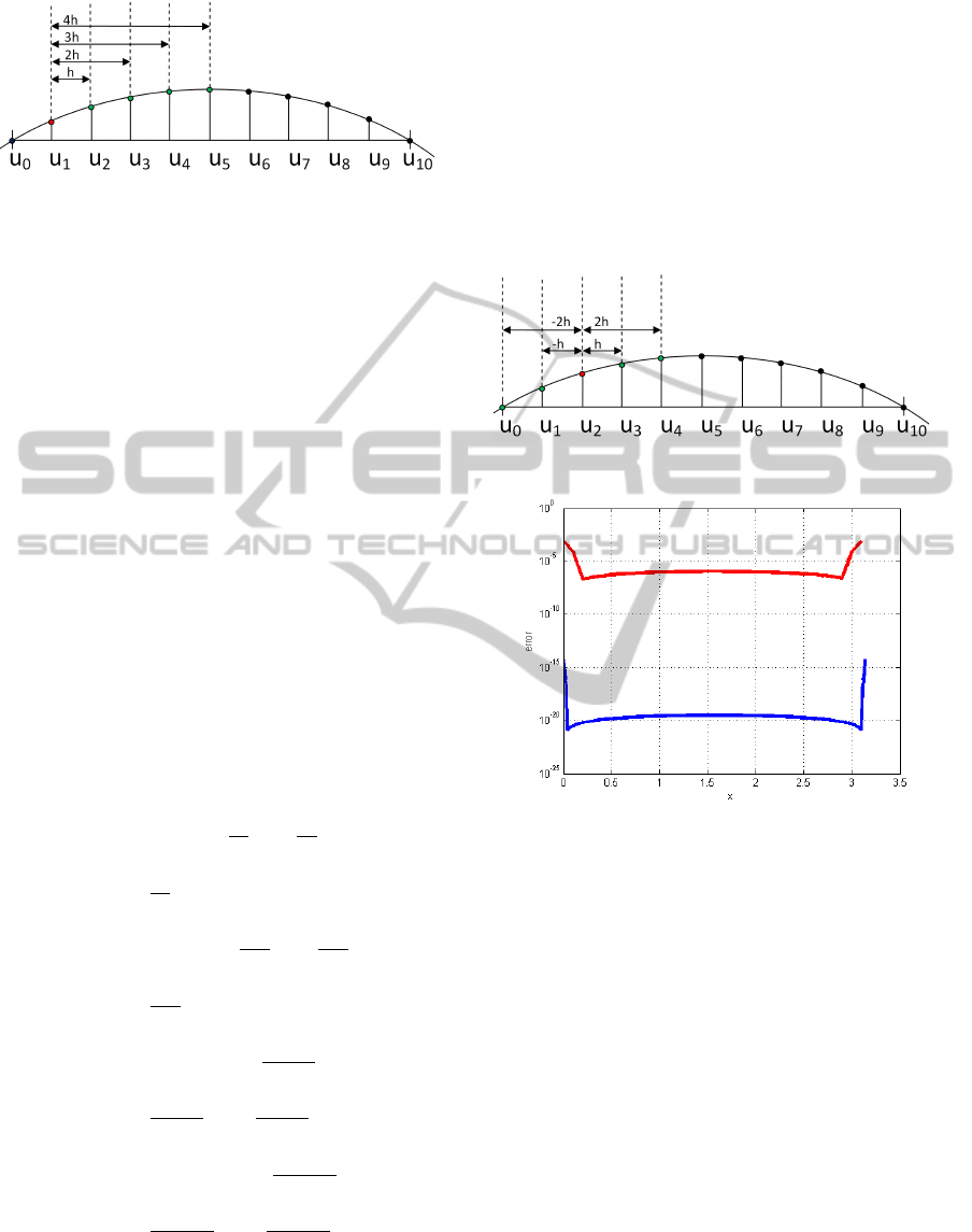
Figure 1: Forward difference formula, point u
1
.
u
2
− u
1
= DU1 + DU2 +
+ DU3 + DU4 (16)
u
3
− u
1
= 2DU1 + 2
2
DU2 +
+ 2
3
DU3 + 2
4
DU4 (17)
u
4
− u
1
= 3DU1 + 3
2
DU2 +
+ 3
3
DU3 + 3
4
DU4 (18)
u
5
− u
1
= 4DU1 + 4
2
DU2 +
+ 4
3
DU3 + 4
4
DU4 (19)
Backward difference formula can be constructed
similarly.
2.4 Symmetrical Difference Formula
Symmetrical difference formula uses the same num-
ber of points from both sides of the current point
(Figure 2). In this case positive and negative steps
are used. Let’s suppose the five-point approximation,
then the Taylor series for the point u
2
can be con-
structed as follows.
u
3
= u
2
+ hu
0
2
+
h
2
2!
u
00
2
+
h
3
3!
u
000
2
+
h
4
4!
u
0000
2
(20)
u
4
= u
2
+ 2hu
0
2
+
2h
2
2!
u
00
2
+
2h
3
3!
u
000
2
+
2h
4
4!
u
0000
2
(21)
u
1
= u
2
+ (−h)u
0
2
+
(−h)
2
2!
u
00
2
+
+
(−h)
3
3!
u
000
2
+
(−h)
4
4!
u
0000
2
(22)
u
0
= u
2
+ (−2h)u
0
2
+
(−2h)
2
2!
u
00
2
+
+
(−2h)
3
3!
u
000
2
+
(−2h)
4
4!
u
0000
2
(23)
It is also possible to denote Taylor series terms as
DU1, DU2, DU3 and DU4.
u
0
− u
2
= −2DU1 + 2
2
DU2 +
− 2
3
DU3 + 2
4
DU4 (24)
u
1
− u
2
= −DU1 + DU2 +
− DU3 + DU4 (25)
u
3
− u
2
= DU1 + DU2 +
+ DU3 + DU4 (26)
u
4
− u
2
= 2DU1 + 2
2
DU2 +
+ 2
3
DU3 + 2
4
DU4 (27)
Figure 2: Symmetrical difference formula, point u
2
.
Figure 3: Symmetrical difference formulas.
2.5 Accuracy of the Calculation
There are two parameters affecting the accuracy. The
first parameter is the integration step. If the smaller
step is used, the resulting solution is more accurate.
The second parameter is the order of the difference
formulas. The higher order is set, the more accurate
solution is obtained.
Figure 4 shows the absolute error between numer-
ical and analytical solution. The upper red function
shows this error for three-point approximation and ten
segments of the string, the lower red function shows
this error for three-point approximation and one hun-
dred segments. This error between numerical and an-
alytical solution can be effectively decreased by an in-
crease in the order of the difference formula. The up-
per blue function represents five-point approximation
and twelve segments. Furthermore, the lower blue
function shows five-point approximation, the string is
divided into one hundred segments.
SIMULTECH2015-5thInternationalConferenceonSimulationandModelingMethodologies,Technologiesand
Applications
156

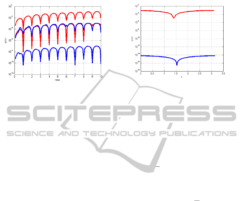
Figure 4: An absolute error between numerical and analyti-
cal solution.
There are also differences between types of differ-
ence formulas. If the forward or backward formulas
are used the same calculation error is obtained, be-
cause both of these formulas are asymmetrical. This
causes the error accumulation. On the other hand,
symmetrical difference formula uses the same number
of points from the both sides, this formula has smaller
calculation error.
Figure 3 shows the absolute error between numer-
ical and analytical solution for symmetrical formulas.
The upper red function shows the absolute error for
five-point approximation (integration step h = 0.1),
the lower blue function for nine-point approximation
(integration step h = 0.01). Note, that these functions
mostly remain at the same level. Higher deviation be-
tween numerical and analytical solution at the ends
of the plotted curves is caused by using asymmetrical
difference formulas.
Figure 5 shows the absolute error between numer-
ical and analytical solution for forward difference for-
mulas, using the same settings as for symmetrical dif-
ference formulas. Note, that the deviation is consider-
ably bigger, because mostly asymmetrical difference
formulas are used.
3 GRADIENT
SUPER-APPROXIMATION
The Gradient super-approximation is a method to cal-
culate gradient of a function of two variables.
Each inner vertex v of a triangulation T is shared
by multiple elements and gradient of a function u(x, y)
in vertex v can differ from element to element.
The idea of the Gradient super-approximation is
to use weighted average and calculate more precise
gradient of a function u(x, y) in vertex v.
Figure 5: Forward difference formulas.
This method is well described in (Dal
´
ık, 2008),
(Dal
´
ık, 2010) and (Dal
´
ık, 2012).
3.1 Triangulation
Triangulation describes a quantization of the area Ω.
Basic elements of triangulation are called elements.
The element can be denoted as t if it is a rectangle.
Each element t is defined by four vertices a
1
, a
2
, a
3
,
a
4
and contains four edges a
1
a
2
, a
2
a
3
, a
3
a
4
and a
4
a
1
.
T
Ω
is called a triangulation of Ω of elements when
the following conditions are fulfilled:
•
S
t ∈ T
Ω
= Ω (the union of all elements covers the
entire area including its border),
• any two different elements have disjoint interiors,
or share an edge, or share a vertex.
A vertex b is a neighbor of a vertex a of a tri-
angulation T when the segment ab is an edge of an
element t of T .
Vertex a is called inner and outer when a ∈ Ω and
a ∈ ∂Ω respectively.
3.2 Interpolant
Let N
n
t
be a bilinear nodal basis function defined for
n-th vertex of an element t (consider only rectangles
with n = 1 . . . 4) of the form N
n
t
(x, y) = a + bx + cy +
dxy. This function is defined by values of all four
element vertices. N
i
t
= 1 for vertex a
i
and N
i
t
= 0 for
all other vertices.
Let’s consider following function as interpolant of
a function u(x, y) on an element t.
Π
t
[u](x, y) =
∑
i=1..4
u(x
i
, y
i
)N
i
(x, y) (28)
where
• t is an element t ∈ T ,
• u is a function of two variables,
AdaptiveSolutionoftheWaveEquation
157

• (x
i
, y
i
) is a position of vertex a
i
,
• u(x
i
, y
i
) is the value of function u in n-th vertex of
element t,
• N
n
is a nodal basis function of n-th vertex of ele-
ment t.
3.3 Ring Around Vertex
Let’s call r
v
= a
1
, a
2
, . . . , a
n
a ring around vertex v,
where a
i
is a vertex of an element of a triangulation
T and va
i
is an edge of an element of a triangulation
T and one of the two following conditions is fulfilled.
1. If v is an inner vertex, then equation (29) is valid.
∠a
n
va
1
+ . . . ∠a
n−1
va
n
= 2π (29)
2. If v is a boundary vertex, then there exists an inner
vertex c and a ring around vertex c denoted as r
c
=
(a
1
, . . . , v, .. . , a
n
). The ring around v is created
swapping c and v vertices. When this condition is
not fulfilled, the Gradient super-approximation is
not applicable.
When this operation is performed, new elements
which are not part of the triangulation are used for
calculation. More details can be found in (Dal
´
ık and
Valenta, 2013).
3.4 Consistency Condition
Each ring r
a
can be transformed into a ring ρ
a
with its
local coordinate system. The vertex a can be moved to
origin of the ring ρ
a
using simple translation. All cal-
culations are performed in this local coordinate sys-
tem. The gradient value is not affected.
The Gradient super-approximation method is
based on the Consistency condition. This condition
says that the partial derivative of a polynomial p(x, y)
in a vertex a must be equal to the weighted aver-
age of partial derivatives of interpolants of a polyno-
mial p(x, y) for all elements from the ring around ver-
tex a for all polynomials p(x, y) of the second order.
Then the error of the gradient is O(h
2
), where h is the
longest edge of an element t (without this operation,
the error is O(h
3
2
)). Formally written in the form
∀p ∈ P
2
,
∂p
∂x
=
∑
∀t∈ρ
a
f
t
∂Π
t
[p]
∂x
(30)
where
• p is a polynomial of the second order,
• ρ
a
is a ring of elements around the vertex a,
• t is an element from the ring of elements around
the vertex a,
• f
t
is a weight value for an element t from the
weight vector w, and f is the weight vector defined
for a ring r
a
.
Because all polynomials of the second order are li-
nearly dependent on a polynomial basis, the second
order polynomial basis is used instead of all polyno-
mials of the second order.
For example, the following basis can be chosen
(31).
B =

1, x, y, xy, x
2
, y
2

(31)
Now let’s consider the Consistency condition for
both derivatives (by x and by y) and all the functions
from the polynomial basis B. The resulting system
of twelve equations can be reduced to the system of
three linear algebraic equations of n variables, where
n is the number of elements in the ring ρ
a
.
It is well known that this system has an infinite
number of solutions, let’s choose the minimal norm
solution.
3.5 Example
In this section a simple example of the Gradient su-
peraproximation is presented on a very simple trian-
gulation containing four rectangles (see Figure 6).
-
6
x
y
b
1
b
2
b
3
b
4
b
5
b
6
b
7
b
8
a = [0, 0]
T
1
T
2
T
3
T
4
Figure 6: Example triangulation with four rectangles.
First, the important values coming out of this tri-
angulation have to be derived.
x
1
= a
x
− b
8
x
(32)
x
3
= b
3
x
− a
x
(33)
y
2
= a
y
− b
2
y
(34)
y
6
= b
6
y
− a
y
(35)
Then the nodal functions N
i
t
have to be derived for
each element.
SIMULTECH2015-5thInternationalConferenceonSimulationandModelingMethodologies,Technologiesand
Applications
158

For example, nodal function for the element T
1
.
T
1
: L
1
1
(x, y) =
1
x
1
y
2
xy (36)
L
2
1
(x, y) = −
1
x
1
y
2
y(x + x
1
) (37)
L
a
1
(x, y) =
1
x
1
y
2
(x + x
1
)(y + y
2
) (38)
L
8
1
(x, y) = −
1
x
1
y
2
x(y + y
2
) (39)
An interpolant template is created for a function u
for each element, for example the element T
1
Π[u]
T
1
(x, y) =u
1
L
1
1
(x, y) + u
2
L
2
1
(x, y)+
+ u
0
L
a
1
(x, y) + u
8
L
8
1
(x, y)
(40)
where u
i
is a value of a function u in a vertex i.
It is necessary to find the weight vector
( f
1
, f
2
, f
3
, f
4
) to fulfill the consistency condition.
f
1
∂Π[p]
T
1
∂x
(a) + . . . + f
4
∂Π[p]
T
4
∂x
(a) =
∂p
∂x
(a)
f
1
∂Π[p]
T
1
∂y
(a) + . . . + f
4
∂Π[p]
T
4
∂y
(a) =
∂p
∂y
(a)
Now all the functions of the basis B are used in
both equations of consistency condition. In fact there
are only four different situations.
Considering p(x, y) = 1, p(x, y) = y or p(x, y) = y
2
for the derivative by x, or p(x, y) = 1, p(x, y) = x or
p(x, y) = x
2
for the derivative by y, equation in the
form 0 = 0 is obtained and therefore can be ignored.
Another situation is for p(x, y) = x for the deriva-
tive by x and p(x, y) = y for the derivative by y. Bi-
linear interpolant Π
t
[p] = p and four same equations
can be created.
∂p
∂x
(a) = f
1
∂p
∂x
(a) + . . . + f
4
∂p
∂x
(a) (41)
∂p
∂x
(a) =
∂p
∂x
(a)( f
1
+ f
2
+ f
3
+ f
4
) (42)
1 = f
1
+ f
2
+ f
3
+ f
4
(43)
Another situation is for p(x, y) = xy for both
derivatives (by x and y), where the derivatives are y
and x. The value of the gradient in point a = [0, 0],
which means that the resulting equation can be ig-
nored.
Different situation is for p(x, y) = x
2
for the
derivative by x and p(x, y) = y
2
for the derivative by
y. It is necessary to calculate all the interpolants for
all four rectangles.
Π[x
2
]
T
1
= Π[x
2
]
T
4
= −x
1
x (44)
Π[x
2
]
T
2
= Π[x
2
]
T
3
= x
3
x (45)
Π[y
2
]
T
1
= Π[y
2
]
T
2
= −y
2
y (46)
Π[y
2
]
T
3
= Π[y
2
]
T
4
= y
6
y (47)
Their appropriate partial derivatives in the point a.
∂Π[x
2
]
T
1
∂x
(a) =
∂Π[x
2
]
T
4
∂x
(a) = −x
1
(48)
∂Π[x
2
]
T
2
∂x
(a) =
∂Π[x
2
]
T
3
∂x
(a) = x
3
(49)
∂Π[y
2
]
T
1
∂y
(a) =
∂Π[y
2
]
T
2
∂y
(a) = −y
2
(50)
∂Π[y
2
]
T
3
∂y
(a) =
∂Π[y
2
]
T
4
∂y
(a) = y
6
(51)
Using these derivatives, two equations of the fol-
lowing form are obtained
f
1
∂Π[x
2
]
1
∂x
(a) + . . . + f
4
∂Π[x
2
]
4
∂x
(a) = 0 (52)
f
1
(−x
1
) + f
2
x
3
+ f
3
x
3
+ f
4
(−x
1
) = 0 (53)
f
1
∂Π[y
2
]
1
∂y
(a) + . . . + f
4
∂Π[y
2
]
4
∂y
(a) = 0 (54)
f
1
(−x
2
) + f
2
(−x
2
) + f
3
y
6
+ f
4
y
6
= 0 (55)
Finally, it is necessary to solve the following sys-
tem of three linear algebraic equations of four vari-
ables and find the solution of the minimal form.
f
1
+ f
2
+ f
3
+ f
4
= 1 (56)
− f
1
x
1
+ f
2
x
3
+ f
3
x
3
− f
4
x
1
= 0 (57)
− f
1
y
2
− f
2
y
2
+ f
3
y
6
+ f
4
y
6
= 0 (58)
4 A POSTERIORI ERROR
ESTIMATION
The a posteriori error estimation is an approach of cal-
culating the error of a solution of the partial differen-
tial equation without knowledge of the analytical so-
lution.
4.1 Calculating a Posteriori Error
Estimation
Because there is no particular formula available, cus-
tom a posteriori error estimation method had to be
created using the Gradient super-approximation.
A posteriori error estimation τ
t
on each element t
of triangulation T is calculated. Element t is denoted
by four vertices which define unique bilinear function
φ(x, y) of two variables of the following form.
φ(x, y) = a + bx + cy + dxy (59)
AdaptiveSolutionoftheWaveEquation
159

It is also possible to calculate gradient of this func-
tion of the form as mentioned below.
(b + dy, c +dx) (60)
It is also necessary to calculate the Gradient super-
approximation presented in section 3. Two bilinear
functions φ
x
and φ
y
that define gradient in the follow-
ing form.
(φ
x
, φ
y
) (61)
Now it is possible to calculate a posteriori error
estimation on element t using the following formula.
τ
t
=
1
|t|
Z
t

∂Π
t
[φ]
∂x
− Π
t
[φ
x
]

2
+
+

∂Π
t
[φ]
∂y
− Π
t
[φ
y
]

2
dxdy
(62)
A posteriori error estimation is the volume be-
tween two curves (for derivative by x and also by y)
which is normalized to the element area (|t|).
This formula is not applicable directly for the
wave equation because it is suitable only for static
boundary value problems (like Laplace’s equation).
The wave equation includes time domain and it is nec-
essary to reflect that.
τ
t
(t) is calculated for each time step and maxi-
mum value is chosen. This is considered as an a pos-
teriori error estimation for element t. Note that this
value τ
t
does not reflect real error of the solution but
it provides the capability to find an element with the
biggest error.
4.2 Using a Posteriori Error Estimation
It is possible to define a method which attempts to
iteratively adapt triangulation to obtain a more pre-
cise solution. The idea behind this method is to start
with very rough triangulation, which produces quite
big error of the solution. A posteriori error estimation
is calculated and elements with big error are identi-
fied. These elements are then replaced by smoother
triangulation, thus more precise solution is obtained
(Ainsworth and Oden, 1997), (Babu
ˇ
ska and Rhein-
boldt, 1978) and (Verf
¨
urth, 1994) .
The advantage is that it is not necessary to update
triangulation uniformly, which means that less equa-
tions are solved and the system can converge faster.
The following algorithm is used:
1. initialize a rough triangulation,
2. solve the wave equation,
3. calculate a posteriori error estimation,
4. find element with big error and update the trian-
gulation,
5. if error is still big enough, continue with point 2.
4.3 Triangulation Update
When a posteriori error estimation is calculated and
the elements with big error are identified, triangula-
tion update is made. Because of using a specific tri-
angulation with the orthogonal edges only, it is nec-
essary to split an element (vertically or horizontally)
and all the elements of the same horizontal (eventu-
aly vertical) position. The scheme is shown on the
following Figure 7.
-
Figure 7: Vertical triangulation update.
5 RESULTS
A posteriori error estimation is used to wave equation
in the following form
∂
2
u
∂x
2
+
∂
2
u
∂y
2
=
∂
2
u
∂t
2
(63)
with the following domain Ω and Dirichlet bound-
ary values on Ω
Ω = h0, 1i × h0, 1i × h0, 1i (64)
u(0, y,t) = u(1, y,t) (65)
u(1, y,t) = sin(πy) (cos(πt) + sin(πt)) (66)
u(x, 0, t) = u(x, 1, t) (67)
u(x, 1, t) = sin(πx) (cos(πt) + sin(πt)) (68)
and following Cauchy initial values.
u(x, y, 0) = sin (πx) + sin(πy) (69)
∂u(x, y, 0)
∂t
= π(sin (πx) + sin(πy)) (70)
It is well known that this equation has the analyti-
cal solution in the following form.
u(x, y,t) =sin(πx)(cos (πt) + sin (πt))
+sin (πy)(cos (πt) + sin(πt))
(71)
The Finite difference method is used to create a set
of ordinary differential equations that were solved
using the Modern Taylor Series Method. The system
is solved for time interval t ∈ h0, 1i.
SIMULTECH2015-5thInternationalConferenceonSimulationandModelingMethodologies,Technologiesand
Applications
160

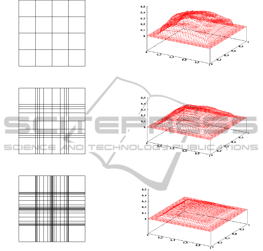
Figure 8: The iterative solution of the wave equation – the
initial triangulation.
Figure 9: The iterative solution of the wave equation – fifth
iteration.
Figure 10: The iterative solution of the wave equation – the
final triangulation.
Triangulations shown on Figures 8, 9 and 10 were
used.
The following Figures 11, 12 and 13 show the ab-
solute error of the solution for time t = 1 for three
chosen triangulations.
6 CONCLUSIONS
A combination of the Modern Taylor Series Method
and the a posteriori error estimation based on the Gra-
dient super-approximation method is presented. A
posteriori error estimation is used for the wave equa-
tion solution.
Figure 11: The absolute error of the solution for t = 1 – the
initial triangulation.
Figure 12: The absolute error of the solution for t = 1 – fifth
iteration.
Figure 13: The absolute error of the solution for t = 1 – the
final triangulation.
The MTSM provides very precise and stable so-
lution of a system of ordinary differential equations
and the a posteriori error estimation provides capabil-
ity to update the triangulation in better way than the
uniform update.
The result is the smaller number of ordinary dif-
ferential equations that needs to be calculated and the
solution is therefore calculated faster.
AdaptiveSolutionoftheWaveEquation
161

ACKNOWLEDGEMENTS
This paper has been elaborated in the framework of
the project New creative teams in priorities of sci-
entific research, reg. no. CZ.1.07/2.3.00/30.0055
(as well as the IT4Innovations Centre of Excellence
CZ.1.05/1.1.00/ 02.0070), supported by Operational
Programme Education for Competitiveness and co-
financed by the European Social Fund and the state
budget of the Czech Republic. The paper includes the
solution results of the international AKTION research
project Number 69p22 and the internal BUT projects
FIT-S-12-1 and FIT-S-14-2486.
REFERENCES
Ainsworth, M. and Oden, J. T. (1997). A posteriori error es-
timation in finite element analysis. Computer Methods
in Applied Mechanics and Engineering, 142(1):1–88.
Babu
ˇ
ska, I. and Rheinboldt, W. C. (1978). A-posteriori er-
ror estimates for the finite element method. Interna-
tional Journal for Numerical Methods in Engineering,
12(10):1597–1615.
Dal
´
ık, J. (2008). Matematika, numerick
´
e metody.
Dal
´
ık, J. (2010). Averaging of directional derivatives in ver-
tices of nonobtuse regular triangulations. Numerische
Mathematik, 116(4):619–644.
Dal
´
ık, J. (2012). Approximations of the partial derivatives
by averaging. Central European Journal of Mathe-
matics, 10(1):44–54.
Dal
´
ık, J. and Valenta, V. (2013). Averaging of gradient in
the space of linear triangular and bilinear rectangular
finite elements. Central European Journal of Mathe-
matics, 11(4):597–608.
Filip Kocina, Ji
ˇ
r
´
ı Kunovsk
´
y, M. M. G. N. A. S. and
ˇ
S
´
atek,
V. (2014). New trends in taylor series based computa-
tions.
Fuchs, G.,
ˇ
S
´
atek, V., Vop
ˇ
enka, V., Kunovsk
´
y, J., and Kozek,
M. (2013). Application of the modern taylor series
method to a multi-torsion chain. Simulation Modelling
Practice and Theory, 2013(33):89–101.
Gabriela Ne
ˇ
casov
´
a, V
´
aclav
ˇ
S
´
atek, J. K. J. C. and Veigend,
P. (2015). Taylor series based differential formulas. In
MATHMOD 2015, Vienna, pages 389–390.
Kunovsk
´
y, J. (1995). Modern Taylor Series Method. Habil-
itation work, Brno University of Technology, Brno.
Kunovsk
´
y, J. (2014). High performance computing - tksl
software.
R. Barrio, M. Rodr
´
ıguez, A. A. and Blesa, F. (2011). Break-
ing the limits: the taylor series method. Applied math-
ematics and computation, 217(20):7940–7954.
R. Barrio, F. B. and Lara, M. (2005). Vsvo formulation
of the taylor method for the numerical solution of
odes. Computers & Mathematics with Applications,
50(1):93–111.
Satek, V., Kunovsk
´
y, J., Kraus, M., and Kopriva, J. (2009).
Automatic method order settings. In Computer Mod-
elling and Simulation, 2009. UKSIM’09. 11th Inter-
national Conference on, pages 117–122. IEEE.
Strikwerda, J. (1989). Finite Difference Schemes and Par-
tial Differential Equations. Chapman & Hall, New
York, NY.
Verf
¨
urth, R. (1994). A posteriori error estimation and adap-
tive mesh-refinement techniques. Journal of Compu-
tational and Applied Mathematics, 50(1):67–83.
SIMULTECH2015-5thInternationalConferenceonSimulationandModelingMethodologies,Technologiesand
Applications
162