
Making the Investigation of Huge Data Archives Possible in an
Industrial Context
An Intuitive Way of Finding Non-typical Patterns in a Time Series Haystack
Yavor Todorov
1
, Sebastian Feller
1
and Roger Chevalier
2
1
FCE Frankfurt Consulting Engineers GmbH, Frankfurter Strasse 5, Hochheim am Main, Germany
2
R&D Recherche et Développement, EDF, Chatou Cedex, France
Keywords: Knowledge Discovery Process, Data Mining, Pattern Recognition, Motif Discovery, Non-trivial Sequence.
Abstract: Modern nuclear power plants are equipped with a vast variety of sensors and measurement devices.
Vibrations, temperatures, pressures, flow rates are just the tip of the iceberg representing the huge database
composed of the recorded measurements. However, only storing the data is of no value to the information-
centric society and the real value lies in the ability to properly utilize the gathered data. In this paper, we
propose a knowledge discovery process designed to identify non-typical or anomalous patterns in time
series data. The foundations of all the data mining tasks employed in this discovery process are based on the
construction of a proper definition of non-typical pattern. Building on this definition, the proposed approach
develops and implements techniques for identifying, labelling and comparing the sub-sections of the time
series data that are of interest for the study. Extensive evaluations on artificial data show the effectiveness
and intuitiveness of the proposed knowledge discovery process.
1 INTRODUCTION
The beginning of the “Information Age” (Goebel,
1999), which can be symbolically identified as the
creation of the World Wide Web on Christmas Day
1990 (McPherson, 2009), sparked an explosion of
interest towards knowledge discovery in databases
(Esling, 2012; Gama, 2010; Fayyad, 1996). The
rapid technological progress of data management
solutions has led to the possibility to store and
access vast amounts of data at practically no cost.
Gigantic databases containing hundreds of petabytes
are something common nowadays.
Informally, the goal of knowledge discovery
applied to databases is to identify a sequence of data
mining tasks designed to analyze and discover
interesting behaviour within the data. Unfortunately,
the progress of data mining was hindered due to a
concern that by employing data mining in an
uninformed way, the findings can be
counterproductive (Fayyad, 1996). Thus, the
development and implementation of knowledge
discovery processes was introduced to ensure that
the final results will be useful for the researcher.
In the past, the mainstream approaches for
turning data into knowledge involved slow,
expensive, and highly subjective manual procedures
for analyzing and understanding the data (Fayyad,
1996). Fortunately, this is not the case anymore
(Goebel, 1999; Kurgan, 2006; Maimon, 2010). Thus,
the knowledge discovery in databases can be seen as
an automatic approach for data analysis that
combines the experience from a variety of scientific
fields, e.g. machine learning, pattern recognition,
statistics, and exploratory data analysis to name a
few. Data mining, on the other hand, is often
misinterpreted and mistaken for knowledge
discovery (Kurgan, 2006). As a result, this work
adopts the definition that is most renown within the
research community which defines knowledge
discovery from datasets as “the nontrivial process of
identifying valid, novel, potentially useful, and
ultimately understandable patterns in data” (Fayyad,
1996). In addition, data mining is understood to be
the central building block of knowledge discovery –
it is the utilization of algorithms and techniques that
aim to provide insight, create models and draw
conclusion for the data.
The proposed knowledge discovery process for
identifying, labelling and comparing non-typical
patterns in time series datasets encompasses some of
the most common data mining tasks such as
569
Todorov Y., Feller S. and Chevalier R..
Making the Investigation of Huge Data Archives Possible in an Industrial Context - An Intuitive Way of Finding Non-typical Patterns in a Time Series
Haystack.
DOI: 10.5220/0005542105690581
In Proceedings of the 12th International Conference on Informatics in Control, Automation and Robotics (ICINCO-2015), pages 569-581
ISBN: 978-989-758-122-9
Copyright
c
2015 SCITEPRESS (Science and Technology Publications, Lda.)

anomaly detection, segmentation, clustering, and
classification.
The rest of the paper is organized as follows.
Chapter 2 introduces the necessary terminology
while chapter 3 briefly overviews the current state in
literature and identifies a reference approach. The
newly proposed knowledge discovery work flow is
described in chapter 4 followed by evaluation and
comparison to the reference method. The paper is
closed with conclusions and ideas for further
research.
2 FOUNDATIONS
This section introduces the necessary terminology
and definitions needed to describe the problem at
hand.
2.1 Definitions and Notation
The aim here is to familiarize the reader with the
definitions and notation that is used throughout this
paper.
Definition 1: Time Series
Let =
∈
be a stochastic process of a simple
random variable defined on a probability
space
Ω,ℋ,ℙ
and arbitrary set, countable or
uncountable. Then, for a fixed ∈ Ω, the realization
=
∈
is called a time series or sequence.
Since in this work we are not so much interested
in the time series data as a whole but on sub-sections
of it, the following definition will come to hand
later.
Definition 2: Sub-sequence
For a given time series =
∈
, a sequence =
∈
is a sub-sequence of if′ ⊆ .
For notational convenience, the following will hold
throughout this paper for time series =
∈
and =
∈
:
−
|
|
≔
|
|
;
−
denotes the
element of the sequence ;
−
denotes the time domain of sequence ;
− max
=max
for 1≤≤
|
|
;
− min
=min
for 1≤≤
|
|
.
A special type of a sub-sequence consists of
contiguous time instance from a time series. This
idea is formalized with the next definition.
Definition 3: Window
Let =
∈
be a sequence of length and =
∈
a sub-sequence of of length. Then, is
called a window in if the following holds:
=
+−1
,
where 1≤≤ and is a fixed index satisfying
1≤≤−+1.
In addition to the notations so far, the following will
be used:
−
denotes the set containing all windows in
of length .
The fact that time series data is characterized by its
continuous nature, high dimensionality and large
size together with the difficulty to define a form of
similarity measure based on human perception
(Goebel, 1999), it is only logical to compare
sequences in an approximate manner.
Definition 4: Distance
Let =
∈
and =
∈
be two time series
of length. The distance between them is given by:
:ℝ
×ℝ
⟶ℝ
.
Often, it is more convenient to work on a
transformed time series than on the original one. The
following transformation of the raw data is
important for the proposed approach.
Definition 5: Normalization
Let =
∈
be a sequence. The function:
Norm
:ℝ⟶ℝ
⟼
−min
max
−min
is called normalization function.
Similarly to the above conventions, the
following notations are to be considered in this
work:
−
=Norm
=Norm
∈
;
− ̅
=Norm
=Norm
.
2.2 Data Mining Tasks
Having introduced the necessary definitions in the
previous section, now we can give a brief overview
of the data mining tasks involved in the proposed
discovery process.
2.2.1 Anomaly Detection
In the context of time series data mining, the goal of
anomaly detection is to discover sub-sequences of a
time series which are considered abnormal.
ICINCO2015-12thInternationalConferenceonInformaticsinControl,AutomationandRobotics
570

Definition 6: Anomaly Detection
Given a time series =
∈
together with some
model of its normal behaviour, the goal of anomaly
detection is to discover all sub-sequences of which
deviate from this normal behaviour.
2.2.2 Representation
One of the fundamental problems in data mining is
how to represent the time series data in such a way
that allows efficient computation on the data.
Typically, one is not so much interested in the global
properties of the time series, but in subsections of it
(Lin, 2002). As a result, segmentation (also known
as time series representation, transformation, or
summarization) is one of the main ingredients in
time series data mining viewed as an intermediate
step of various tasks, such as indexing, clustering,
classification, segmentation and anomaly detection.
This stems from the fact that often time series are
too big to be analyzed and the utilization of time
series representations allows more efficient
computation by reducing the size of the data while
preserving its fundamental shape and characteristic.
This transformation process can be defined as
follows:
Definition 7: Representation
Given a sequence =
∈
of length, the goal
of representation is to find a transformation function
of given by:
:ℝ
⟶ℝ
⟼
which reduces and closely approximates :
≪,
|
−
|
≤
with ∈ℝ
some preselected threshold value.
2.2.3 Clustering
Clustering is perhaps the most common task in the
unsupervised learning problem (Gama, 2010) which
aims at grouping the elements from a dataset into
clusters by maximizing the inter-cluster variance
while minimizing intra-cluster variance:
Definition 8: Clustering
Let be a time series database and - a distance
measure. The goal of clustering is to construct a set
=
of clusters such that:
=
:
∈
and for ever
,
,:
,
∈
∧
∈
holds:
,
≫
,
.
2.2.4 Classification
Classification is the natural counterpart of clustering
in the supervised learning scenario. Contrary to
clustering where no information is present in the
data regarding class belongings, the main objective
here is to learn what separates one group from
another:
Definition 9: Classification
Let be a time series database and =
a set
of classes. The goal of classification is for every ∈
to assign it to one
.
3 BACKGROUND
Starting from datasets containing historic recordings
of a technical system such as a steam turbine, a non-
typical pattern discovery process should review all
interesting events contained in this dataset. These
events include machine failures, changes in
operating mode and all other patterns that
significantly deviate from normal operation.
The problem of determining parts in time series
data that somehow defy our expectations of normal
structure and form is known by many names in the
literature – from “surprises” through “faults” to
“discords”. Independent of the term used, most
existing knowledge discovery algorithms and
procedures approach this problem by using a brute
force algorithm, known as sliding window
technique, for building the set
for a given time
series and some preselected value (Lin, 2002; Fu,
2005; Keogh, 2002; Lin, 2005). The next step taken
normally involves dimensionality reduction and
discretization. Arguably, one of the most referenced
and widely used techniques for accomplishing this
task is the symbolic aggregate approximation (SAX)
(Lin, 2005; Lin, 2003) which relies on piecewise
aggregate approximation as an intermediate
dimensionality reduction step (Yi, 2000; Keogh,
2001). Thus, we give a brief overview of these
procedures.
3.1 Piecewise Aggregate
Approximation (PAA)
A member of the category of approximations that
represent the time series directly in the time domain,
PAA is one of the most popular choices for
representation and is defined as follows.
MakingtheInvestigationofHugeDataArchivesPossibleinanIndustrialContext-AnIntuitiveWayofFinding
Non-typicalPatternsinaTimeSeriesHaystack
571

Definition 10: PAA
Given a sequence =
∈
of length, the
element of the PAA representation
=
∈
in
dimensional space is given by:
=
with =
−1
+1 and =
.
Despite its simplistic character (figure 1), it was
shown in (Keogh and Kasetty, 2002) that this
method is competitive with the more sophisticated
approximation techniques such as Fourier transforms
and wavelets.
Figure 1: Piecewise aggregate approximation (PAA).
3.2 Symbolic Aggregate
Approximation (SAX)
After employing the PAA transformation, each
segment of the compressed time series is mapped to
a symbol string. The construction of the “alphabet”
is performed in such a way that every “letter” is
equiprobable. To accomplish this task, the y-axis is
divided into equiprobable regions defining a set of
breakpoints (Lin, 2003):
Definition 11: Breakpoint
The real-valued numbers in an order set =
,…,
are said to be breakpoints if the area
under a
0,1
Gaussian curve from
to
is
equal to
1
with
=−∞ and
=+∞.
Once the breakpoints for the desired alphabet length
are found, all PAA segments that are below
are
mapped to letter “a”, between
and
to letter “b”
and so on. Formally (Lin, 2003):
Definition 12: Word
Let
denote the
letter of the selected alphabet
(i.e.
=,
=, etc.) and =
∈
be a
sequence of length. Furthermore, assume
=
∈
is the PAA approximation of length.
Then, is mapped into word
as follows:
=
⟺
≤
.
This idea is visualized next.
Figure 2: Symbolic aggregate approximation (SAX).
Subsequently, the discovery of the abnormal
patterns is accomplished by examining their
expected frequency. More formally (Lin, 2005):
Definition 13: Frequency
Let be a time series and - a pattern. Then, the
frequency of occurrence of in, denoted
, is
the number of occurrences of in divided by the
total number of patterns found in denoted by
max
.
Definition 14: Support
Let and be two time series. Then, the measure
indicating how a pattern differs from one time
series to another is called support and is given as:
Sup
=
−
max
,
.
Then, a pattern is considered to be overrepresented
in ifSup
0. On the other hand, ifSup
0,
then the pattern is believed to be underrepresented
in.
The obvious limitation in the aforementioned
work flow is the inability of PAA to precisely
enough mimic the dynamics of highly volatile
regions of the time series as will be demonstrated
later. In addition, modifying this work flow to take
into account patterns of different resolutions is
everything but a trivial task. Furthermore,
determining the abnormality of a pattern using the
support can be difficult for new abnormal patterns
since the frequency in this case will not be
representative.
4 NOVEL NON-TYPICAL
PATTERN DISCOVERY
APPROACH
Supplementary to the description of the problem at
hand in the previous section, we require that the
patterns should successfully be exploited from
univariate and multivariate process data and the
discovery process should run in the form of an
unsupervised learning method. This means that the
user does not have to supply any additional
information besides the historical data. To establish
ICINCO2015-12thInternationalConferenceonInformaticsinControl,AutomationandRobotics
572
a correct identification of cause and reactive
causality, user prompts should be limited to general
questions only, such as selection of relevant
parameters and specification of input and output
signals. The problem is further obscured by the fact
that a key goal is the identification of unknown
patterns from different resolutions and distortions
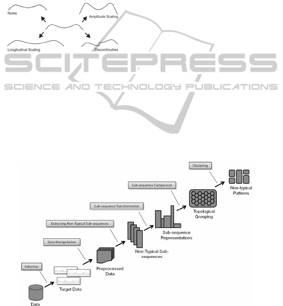
(see figure 3). The idea behind the proposed non-
typical pattern discovery process is visualized in
figure 4.
Figure 3: Distortions.
4.1 Selection
Coming from a time series database, the goal
here is to select which time series should be
considered for the unsupervised discovery of
abnormal patterns. Depending on this selection, the
subsequent steps in the process will either be
concerned with univariate or multivariate patterns.
However, it should be noted that even techniques
designed for finding univariate patterns can easily be
extended to multivariate patterns as shown in
(Minnen, 2007).
4.2 Data Manipulation
Time series data occurs frequently in business
applications and in science. Some well-known
examples include temperatures, pressures,
vibrations, emission, average fuel consumption, and
many other quantities that are part of our everyday
life. Be that as it may, as pointed out in (Keogh,
1998), classic machine learning and clustering
algorithms utilized on time series data do not
provide the expected results due to the nature of the
time series data.
Besides the standard techniques for pre-
processing the raw data (e.g., cleaning the data,
outlier removal, testing for missing values, etc.), the
time series here are further processed to be suitable
for extracting abnormal sub-sections from them.
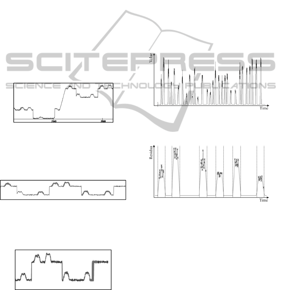
4.2.1 Compression
Often the industrial data encompasses several
decades where the measurements are taken as often
as once per second. Thus, removing redundant
information and reducing the length of the data is of
upmost importance.
Although any compression algorithm can be
applied here (e.g., PAA), we employ the
multidimensional compression technique introduced
in (Feller, 2011) which is based on the perceptually
important points algorithm pioneered in (Chung,
2001) and exemplified in figure 5.
Figure 4: Work flow of the proposed non-typical pattern discovery process.
MakingtheInvestigationofHugeDataArchivesPossibleinanIndustrialContext-AnIntuitiveWayofFinding
Non-typicalPatternsinaTimeSeriesHaystack
573
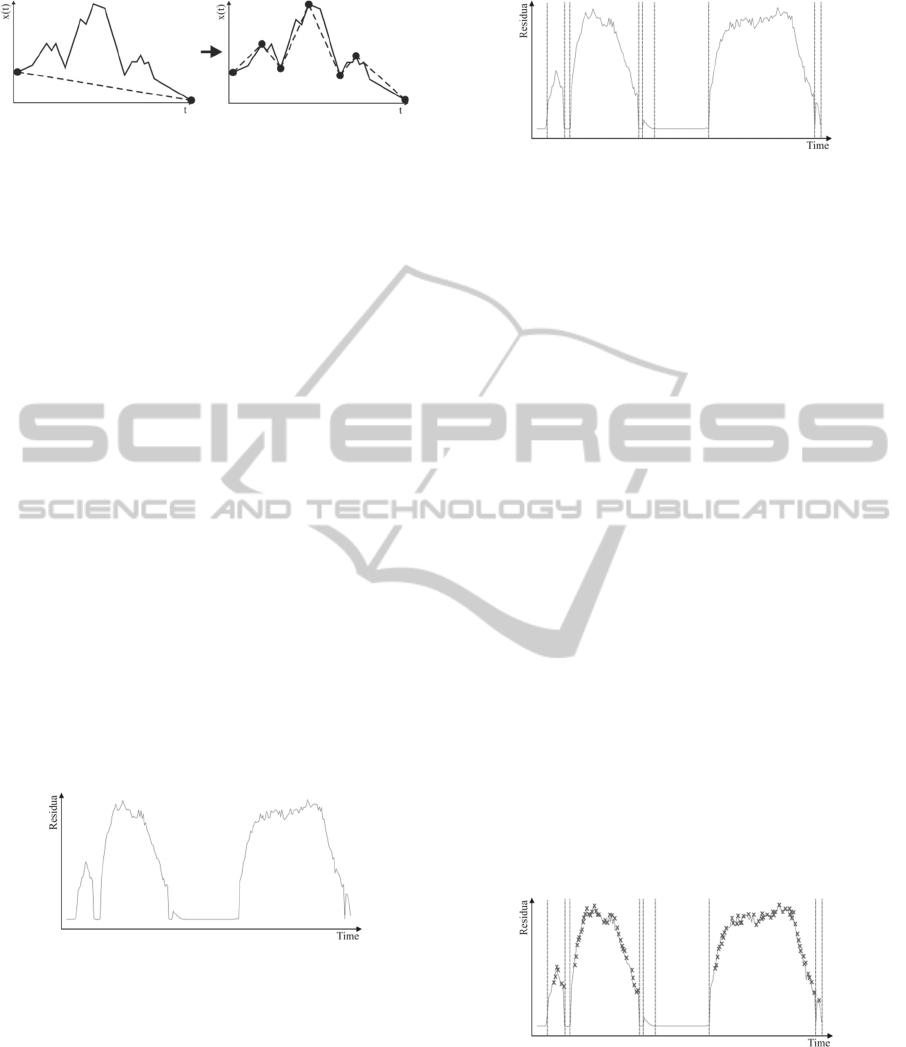
Figure 5: Perceptually important points (PIPs).
This choice was made due to the efficiency shown
by the algorithm on datasets exhibiting strong
stochastic dependencies (Feller, 2011).
4.2.2 Generating Residua
Since our goal is discovering the abnormal patterns,
contrary to the traditional work flow, our approach
searches for non-typical segments on the residual
signal instead of the original raw data. This idea is
motivated first and foremost by the desire to detect
patterns of different lengths. In addition, given a
well-fitted anomaly detection model, it is reasonable
to expect that the residuals for the different signals
will be uncorrelated as long as no anomaly is present
(Feller, 2013). Thus, the discovery can be executed
in a univariate manner – signal by signal. Once the
univariate non-typical patterns are found, they can
be merged into multidimensional patterns using a
collision matrix (Minnen, 2007). Thus, the next step
in our approach is to generate the multidimensional
residual signal by using a data-driven condition
monitoring method. A possible outcome is depicted
in figure 6. (Feller, 2013) provides a complete and
detailed analysis on this subject together with
numerous modifications on the state-of-the-art
algorithms leading to improved detection accuracy.
Figure 6: Residual signal.
4.3 Extracting Non-typical
Sub-sequences
Assuming the anomaly detection model is well-
suited, the residua are centered around zero and any
significant deviations indicate some abnormality. In
order to identify normal and abnormal intervals on
the residual signal, a structural break detection
algorithm can be employed. Continuing the example
from last section, a possible outcome of structural
breaks detection is shown next.
Figure 7: Structural breaks detection – vertical lines
indicate breaks.
Once these structural breaks are identified, the
pattern candidates can be defined. A pattern
candidate is defined to be a segment of the residual
curve between two consecutive structural breaks.
The cornerstone of this procedure is the
structural breaks detection. Although any reasonable
algorithm will be sufficient, the algorithm of choice
for this work is based on Chernoff’s bounds since it
was shown in (Pauli, 2013) that it outperforms with
respect to performance and diagnostic capabilities
some well-known algorithms like sequential
probability ratio test (SPRT) (Takeda, 2010; Kihara,
2011), Chow test (Chow, 1960) and exact bounds.
The interested reader is welcomed to review this
technique in details in (Pauli, 2013).
However, we are interested only in the non-
typical patterns. Thus, a separation between healthy
and abnormal pattern candidates is needed. The
classification, or distinction, between trivial and
non-trivial pattern candidates is accomplished using
a technique called sequential probability ratio test
(Wald, 1945) that was developed by Wald in the
early 1940’s and is primarily used for sequential
hypothesis testing of stationary time series data. This
technique is used to generate degradation alarms on
the residual data. After this, a simple rule for
abnormality is if an alarm is present in a pattern
candidate, then it is identified as non-typical (similar
to figure 8).
Figure 8: Typical (no alarms) and non-typical (alarms as
crosses) pattern candidates.
In the consequent sections, it is assumed that a
set of non-typical pattern candidates was found in
this step denoted by:
=
∈
where I
is the index set of P and p
=p
∈
.
ICINCO2015-12thInternationalConferenceonInformaticsinControl,AutomationandRobotics
574

4.4 Sub-sequence Transformation
As noted previously, the pattern candidates may
suffer from different distortions which may or may
not be relevant for the study (see figure 3). Since
noise distortion is always relevant and to some
extent present, and also computational efficiency is
needed, segmentation is used as pre-processing on
the pattern candidates.
4.4.1 Representation
Time series representation is often seen as a trade-
off between accuracy and efficiency. With this in
mind, some of the commonly used time series
approximation techniques, such as moving averages,
best-fitting polylines and sampling, have the
drawback of missing important peaks and troughs
(Man, 2001) and distorting the time series. Thus, a
great number of high-level time series
representations have been introduced in the literature
in an attempt to find equilibrium between accuracy
and efficiency (Fu, 2011) including PAA, adaptive
piecewise constant approximation (APCA)
(Chakrabarti, 2002), piecewise linear segmentation
(PLA/PLR) (Pavlidis, 1974), SAX, discrete Fourier
transform (DFT) (Agrawal, 1993), discrete wavelet
transform (DWT) (Bronshtein, 2004), singular value
decomposition (SVD) (Press, 2007), and
perceptually important points (PIP) (Chung, 2001).
The latter is a considerable factor within the data
mining community. More specifically, PIP
identification process has been used in the recent
years for representation (Fu, 2001), clustering (Fu
and Chung, 2001), pattern discovery, prediction,
classification (Zhang, 2010), compression (Feller,
2011), and segmentation. This combined with PIP’s
ability to successfully capture the shape of a time
series motivates our decision to utilize this algorithm
in our work. As a result, the non-typical pattern
candidates are compressed using PIP procedure:
=
∈
where
=PIP
represents the PIP compression
of
.
4.4.2 Transformation
The next stage of the transformation process needs
to differentiate between different cases of distortion
relevance. For the sake of brevity, in the following
we consider the most challenging case where only
the general form of the pattern is relevant – i.e. all
the distortions are irrelevant and two patterns are
considered similar if their overall shape is identical.
Definition 15: Transformation – General Form
For =
,
∈
, the transformation of the pattern
candidate is achieved using the following function:
Trans
:ℝ
⟶ℝ
⟼
̅
̅
where ̅
̅
indicates that the value and the time are
normalized.
In other words, the transformation consists in
normalizing the values of
as well as the values
of
.
As a result, the pattern candidates will have
points between 0 and 1 on both axes as shown next.
4.5 Sub-sequence Comparison and
Topological Grouping
This step of the proposed knowledge discovery
process aims at grouping the non-typical pattern
candidates together. However, two questions arise.
First, what distance measure should be used for
comparison. Second, how to create the grouping
without a priori knowledge of class belonging.
4.5.1 Comparison
The majority of the data mining tasks entail some
kind concept of similarity between time series
objects. Hence, the similarity of the compressed and
transformed non-trivial pattern candidates is defined
next.
Definition 16: Sequences Maximum
Let =
∈
and =
∈
be two sequences
of length. Then, the maximum of and is
defined as:
Max
,
:ℝ
×ℝ
⟶ℝ
,
⟼max
,
The idea is illustrated with the next figures. Figure 9
depicts two compressed and transformed sub-
sequences and figure 10 shows their Max depicted in
bold.
Figure 9: Two compressed and transformed sub-
sequences.
MakingtheInvestigationofHugeDataArchivesPossibleinanIndustrialContext-AnIntuitiveWayofFinding
Non-typicalPatternsinaTimeSeriesHaystack
575

Figure 10: Max(bold line) of two compressed and
transformed sub-sequences.
Contrary to the previous definition, the
overlapping between two sequences is given as
follows.
Definition 17: Sequences Overlapping
Let =
∈
and =
∈
be two sequences
of length. Then, the overlap of and is defined
as:
Overlap
,
:ℝ
×ℝ
⟶ℝ
,
⟼min
,
The shaded area in figure 11 represents the overlap
between the two compressed and transformed sub-
sequences from figure 9.
Figure 11: Overlap(bold line) of two compressed and
transformed sub-sequences.
It should be noted that the last two definitions
present results for the simplified case when the
sequences are of the same size and the same time
domain. For the compressed and transformed non-
typical pattern candidates this is not the case.
However, using linear interpolation the union and
overlapping is found easily in linear time.
Now we can define the similarity between two
sub-sequences.
Definition 18: Similarity
Let
and
be two compressed and transformed
non-typical pattern candidates. Then, the similarity
between them is given by:
Sim
,
=
AreaOverlap
,
AreaMax
,
,
where Area
represents the area under .
In other words, the similarity between the two
pattern candidates is the percentage of their overlap.
Also, note that Sim
∙,∙
∈
0,1
and the closer the
value to 1, the more similar the sub-sequences. In
addition, the last definition can be used to formulate
the notion of distance.
Definition 19: Distance
Let
and
be two compressed and transformed
non-typical pattern candidates. Then, the distance
between them is defined as:
Dist
,
=1−Sim
,
.
Note that the distance measure given by definition
19 is a metric.
4.5.2 Grouping
The previous section showed how the pattern
candidates can be compared regardless of their
length and the distortions they are suffering from.
For the construction of the grouping from the pattern
candidates, a modified version of the Kohonen Self-
Organizing Map (SOM) (Kohonen, 2001) is used
where the distance metric for determining the best
matching unit for a given sub-sequence is given by
definition 19. The lattice of the training network is
visualized in figure 12 using unified distance matrix
(Vesanto, 2000).
4.6 Clustering
Once the training of the self-organizing map is
completed, by either achieving some preselected
number of iterations or the overall error is below a
user-defined threshold value, the non-typical
patterns can be generated by clustering the lattice of
the network. Initially, the optimal number of clusters
on the lattice is determined using the Davies-
Bouldin cluster validation index described in
(Arbelaitz, 2013) and then a clustering algorithm is
employed to create the clusters (e.g., k-means). A
possible clustering is depicted in figure 13.
Figure 12: U-Matrix – white color signifies small distance,
while black color indicates large distance between
prototypes.
ICINCO2015-12thInternationalConferenceonInformaticsinControl,AutomationandRobotics
576

Figure 13: Lattice clustering.
The construction of the pattern centers, or motifs,
can be accomplished by averaging all members
within a cluster weighted by their hits (number of
times a specific prototype was a best matching unit).
Definition 20: Non-Typical Pattern
Let
be a cluster found on the lattice of the SOM.
Then, the non-typical patterns can be constructed as:
=
∈
where
=
.
∈
The value
represents the weighting coefficient
for prototype and is given by:
=
with
indicating the number of hits for prototype
and
is the total number of hits within cluster
:
=
∈
.
5 EVALUATION
In this section, the performance of the proposed
approach for discovering abnormal patterns is
compared to the SAX-based technique explained in
section 3.
5.1 Experimental Setup
In computer programming, unit tests are used to test
the correctness of a procedure by using artificial data
for which the outcome is known. Similarly, we
define the following artificial scenario. The first
1500 records of the artificial data presented in figure
14 represent the healthy state of a system and will be
used as a reference, or training, time series.
Figure 14: Artificial data with patterns.
Table 1: For a window length of 40, PAA dimension of 4,
and alphabet size of 6, the SAX-based method results in
21 of 30 patterns discovered whereby 20 of 30 identified
precisely, but also featuring 2 false positives.
Rank
# 1 2 3 4 5 6 7 8 9 10 Hits
…
18 TT O Y Y
19 TT
20 HS O Y Y
21 DT Y Y
22 TT O O
…
F 1 1 2
Table 2: For a window of length of 40, PAA dimension of
5, and alphabet size of 6, the SAX-based method results in
15 of 30 patterns discovered whereby only 3 of 30
identified precisely. In addition, 1 false positive was
present.
Rank
# 1 2 3 4 5 6 7 8 9 10 Hits
…
18 TT O O
19 TT
20 HS O O
21 DT O O
22 TT
…
F 1 1
Table 3: For a window of length 60, PAA dimension of 4,
and alphabet size of 6, the SAX-based method results in
17 of 30 patterns discovered whereby none was identified
precisely. Furthermore, two false positives were present.
Rank
# 1 2 3 4 5 6 7 8 9 10 Hits
…
18 TT O O
19 TT
20 HS O O
21 DT O O O
22 TT O O
…
F 1 1 2
The rest of the data, roughly 3000 records, will be
used for pattern discovery. Three types of patterns
MakingtheInvestigationofHugeDataArchivesPossibleinanIndustrialContext-AnIntuitiveWayofFinding
Non-typicalPatternsinaTimeSeriesHaystack
577
are used – head and shoulders (HS), triple top (TT)
and double top (DT) (see figure 3.4 in (Fu, 2001)).
Each pattern is added 10 times in the time series
together with some distortions. However, the length
of all patterns is kept fixed at 40 records in order to
give competitive edge to the SAX-based algorithm.
Note that for our approach, the length of a pattern is
irrelevant and as such patterns of different
resolutions can be found.
5.2 Results
Tables 1 through 3 present the results obtained using
the SAX-based approach. In each table, the rows
represent the 30 patterns inside the time series (only
patterns 18 to 22 are shown for compactness) while
the columns are the 10 most surprising patterns
found by SAX. The letter “O” indicates that the
corresponding SAX surprising pattern is
“overlapping” the real pattern. An example of this is
displayed next.
Figure 15: “O” - overlapping patterns (SAX-based pattern
is depicted in bold).
As seen from the figure, the pattern found by the
SAX-based approach is overlapping the real pattern
to some extend – not a complete match. On the other
hand, “Y” indicates a total hit (figure 16).
Figure 16: “Y” - matching patterns (SAX-based pattern is
depicted in bold).
In addition, a false alarm (the “F” row in the tables)
is considered patterns missing completely the real
ones (figure 17).
Figure 17: False patterns (SAX-based pattern is depicted
in bold).
It can be concluded from the results presented
above that the SAX-based approach is fairly
accurate given an optimal configuration (in this case
40 window length, 4 dimension for PAA, 6 alphabet
size). However, it is clear that even slight changes in
this configuration (changing the PAA dimension
from 4 to 5, or changing the alphabet size from 6 to
4, or using a sliding window of 60) degrades the
results greatly. Moreover, even for the optimal
configuration, the patterns found are mixed – e.g., in
table 1, rank 10 surprising pattern mixes together all
patterns (18 is TT, 20 is HS, 21 is DT).
Next follows the analysis of the proposed work
flow. Figure 18 portrays the residua obtain from an
anomaly detection algorithm (in this case an
improvement of the Nadaraya-Watson-Estimator
(Feller, 2013) was used).
Figure 18: Residual line.
After this, the structural breaks detection and the
SPRT deliver results similar to figure 19.
Figure 19: Structural breaks and SPRT alarms marked by
vertical lines and crosses respectively.
For the construction of the non-typical patterns, a
SOM was used with the following specifications:
− Number of iterations = 10000
− Lattice dimension = 50x50
− Neighbourhood kernel = Gaussian
− Start / End learning rate = 0.8 / 0.003
− Start / End radius = 30 / 5
The resulting trained lattice is shown next.
ICINCO2015-12thInternationalConferenceonInformaticsinControl,AutomationandRobotics
578
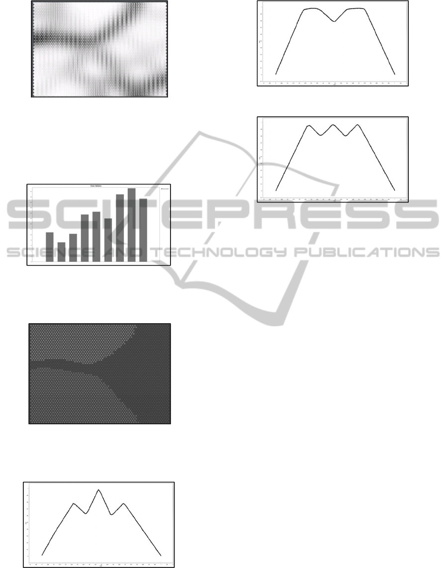
Figure 20: U-Matrix of trained SOM.
For determining the optimal number of clusters on
the lattice, the Davies-Bouldin index was used. As
seen in figure 21, the index has it minimum value at
3 as expected.
Figure 21: Davies-Bouldin cluster validity index for
k=2,..., 10.
Applying k-means with k=3 yields:
Figure 22: Clustered lattice with 3 clusters.
The corresponding non-typical patterns are found
using definition 20 and listed below.
Figure 23: Centroid of cluster 1.
Figure 24: Centroid of cluster 2.
Figure 25: Centroid of cluster 3.
In addition, all non-trivial pattern candidates were
successfully mapped to the corresponding clusters.
6 CONCLUSIONS AND FUTURE
WORK
It was described and illustratively shown how with
the help of an anomaly detection algorithm and a
flexible compression and transformation technique,
non-typical patterns can be identified, labelled and
compared. Applied to the problem of discovering
abnormal patterns, the proposed work flow
outperformed the standard literature approaches such
as SAX-based methods. In addition, the suggested
knowledge discovery process does not need any a
priory knowledge regarding the hidden patterns and
therefore is suitable for non-domain expert users.
One of the bottlenecks for analyzing huge
amounts of data with the proposed discovery process
is the PIP compression with a running time
of
. Therefore, a research in this direction will
be worthwhile.
Finally, further comparison and evaluation on
real industrial data should give supplementary
insight on how the proposed non-typical pattern
discovery process performs compared to the
standard approaches.
REFERENCES
Goebel, M., Gruenwald, L., 1999. A survey of data mining
MakingtheInvestigationofHugeDataArchivesPossibleinanIndustrialContext-AnIntuitiveWayofFinding
Non-typicalPatternsinaTimeSeriesHaystack
579

and knowledge discovery software tools. In ACM
SIGKDD Explorations Newsletter, pp. 20-33.
McPherson, S., 2009. Tim Berners-Lee: inventor of the
World Wide Web, USA Today Lifeline Biographies.
Esling, P., Agon, C., 2012. Time-series data mining. In
ACM Computing Surveys, pp. 12:1-12:34.
Gama, J., 2010. Knowledge discovery from data streams,
CRC Press.
Fayyad, U., Piatetsky-Shapiro, G., Smyth, P., 1996. From
data mining to knowledge discovery in databases. In
AI Magazine, pp. 37-54.
Kurgan, L., Musilek, P., 2006. A survey of knowledge
discovery and data mining process models. In The
Knowledge Engineering Review, pp. 1-24.
Maimon, O., Rokach, L., 2010. Data mining and
knowledge discovery handbook, Springer, 2
nd
edition.
Lin, J., Keogh, E., Lonardi S., Patel, P., 2002. Finding
motifs in time series. In The 8
th
ACM International
Conference on Knowledge Discovery and Data
Mining, pp. 53-68.
Fu, T., Chung, F., Luk, R., Ng, V., 2005. Preventing
meaningless stock time series pattern discovery by
changing perceptually important point detection. In
Fuzzy Systems and Knowledge Discovery, 2
nd
International Conference, pp. 1171-1174.
Keogh, E., Lonardi, S., Chiu, B., 2002. Finding surprising
patterns in a time series database in linear time and
spac. In Proceedings of the 8
th
ACM SIGKDD
International Conference on Knowledge Discovery
and Data Mining, pp. 550-556.
Lin, J., 2005. Discovering unusual and non-trivial
patterns in massive time series databases, University
of California, Riverside.
Lin, J., Keogh, E., Lonardi, S., Chiu, B., 2003. A symbolic
representation of time series, with implications for
streaming algorithms. In Proceedings of the 8
th
ACM
SIGMOD Workshop on Research Issues in Data
Mining and Knowledge Discovery, pp. 2-11.
Yi, B., Faloutsos, C., 2000. Fast time sequence indexing
for arbitrary Lp norms. In Proceedings of the 26
th
International Conference on Very Large Data Bases,
pp. 385-394.
Keogh, E., Chakrabarti, K., Pazzani, M., Mehrotra, S.,
2001. Dimensionality reduction for fast similarity
search in large time series databases. In Knowledge
and Information Systems, pp. 263-286.
Keogh, E., Kasetty, S., 2002. On the need for time series
data mining benchmarks: a survey and empirical
demonstration. In Proceedings of the 8
th
ACM
SIGKDD International Conference on Knowledge
Discovery and Data Mining, pp. 102-111.
Minnen, D., Isbell, C., Essa, I., Starner, T., 2007.
Detecting subdimensional motifs: an efficient
algorithm for generalized multivariate pattern
discovery. In 7th IEEE International Conference on
Data Mining, pp. 601-606.
Keogh, E., Pazzani, M., 1998. An enhanced representation
of time series which allows fast and accurate
classification, clustering and relevance feedback. In
Proceedings of the 4
th
International Conference on
Knowledge Discovery and Data Mining, pp. 239-241.
Feller, S., Todorov, Y., Pauli, D., Beck, F., 2011.
Optimized strategies for archiving multidimensional
process data: building a fault-diagnosis database. In
ICINCO, pp. 388-393.
Chung, F., Fu, T., Luk, R., Ng, V., 2001. Flexible time
series pattern matching based on perceptually
important points. In International Joint Conference on
Artificial Intelligence Workshop on Learning from
Temporal and Spatial Data, pp. 1-7.
Feller, S., 2013. Nichtparametrische Regressionsverfahren
zur Zustandsüberwachung, Zustandsdiagnose und
Bestimmung ener optimalen Strategie zur Steuerung
am Beispiel einer Gasturbine und einer
Reaktorkühlmittelpumpe, Institu für Theoretische
Physik de Universität Stuttgart.
Pauli, D., Feller, S., Rupp, B., Timm, I., 2013. Using
Chernoff’s bounding method for high-performance
structural break detection and forecast error reduction.
In Informatics in Control, Automation and Robotics,
pp. 129-148.
Takeda, K., Hattori, T., Izumi, T., Kawano, H., 2010.
Extended SPRT for structural change detection of time
series based on a multiple regression model. In
Artificial Life and Robotics, pp. 417-420.
Kihara, S., Morikawa, N., Shimizu, Y., Hattori, T., 2011.
An improved method of sequential probability ratio
test for change point detection in time series. In
International Conference on Biometrics and Kansei
Engineering (ICBAKE), pp. 43-48.
Chow, G., 1960. Tests of equality between sets of
coefficients in two linear regressions. In
Econometrica, pp. 591-605.
Wald, A., 1945. Sequential tests of statistical hypotheses.
In The Annals of Mathematical Statistics, pp. 117-186.
Man, P., Wong, M., 2001. Efficient and robust feature
extraction and pattern matching of time series by a
lattice structure. In Proceedings of the 10
th
International Conference on Information and
Knowledge Management, pp. 271-278.
Fu, T., 2011. A review on time series data mining. In
Engineering Applications of Artificial Intelligence, pp.
164-181.
Chakrabarti, K., Keogh, E., Mehrotra, S., Pazzani, M.,
2002. Locally adaptive dimensionality reduction for
indexing large time series databases. In ACM
Transactions on Database Systems (TODS), pp. 188-
228.
Pavlidis, T., Horowitz, S., 1974. Segmentation of plane
curves. In IEE Transactions on Computers, pp. 860-
870.
Agrawal, R., Faloutsos, C., Swami, A., 1993. Efficient
similarity search in sequence databases. In
Proceedings of the 4
th
International Conference on
Foundations of Data Organization and Algorithms,
pp. 69-84.
Bronshtein, I., Semendyayev, K., Musiol, G., Mühlig, H.,
2004. Handbook of mathematics, Springer, 4
th
edition.
ICINCO2015-12thInternationalConferenceonInformaticsinControl,AutomationandRobotics
580

Press, W., Teukolsky, S., Vetterling, W., Flannery, B.,
2007. Numerical recipes, Cambridge University Press.
Fu, T., 2001. Time series pattern matching, discovery &
segmentation for numeric-to-symbolic conversion, The
Hong Kong Polytechnic University.
Fu, T., Chung, F., Ng, V., Luk, R., 2001. Pattern discovery
from stock time series using self-organizing maps. In
KDD Workshop on Temporal Data Mining, pp. 26-29.
Zhang, Z., Jiamg, J., Liu, X., Lau, R., Wang, H., Zhang,
R., 2010. A real time hybrid pattern matching scheme
for stock time series. In Proceeding of the 21
st
Australasian Conference on Database Technologies,
pp. 161-170.
Kohonen, T., 2001. Self-organizing maps, Springer, 3
rd
Edition.
Vesanto, J., Alhoniemi, E, 2000. Clustering of the self-
organizing map. In IEEE Transactions on Neural
Networks, pp. 586-600.
Arbelaitz, O., Gurrutxaga, I, Muguerza, J., Perez, J.,
Perona, I., 2013. An extensive comparative study of
cluster validity indices. In Pattern Recognition, pp.
243-256.
MakingtheInvestigationofHugeDataArchivesPossibleinanIndustrialContext-AnIntuitiveWayofFinding
Non-typicalPatternsinaTimeSeriesHaystack
581
