Computational Correction for Imaging through Single Fresnel Lenses

Artem Nikonorov

1,2

, Sergey Bibikov

1,2

, Maksim Petrov

, Yuriy Yuzifovich

and Vladimir Fursov

1,2

Samara State Aerospace University, 34 Moskovskoe shosse, Samara, Russian Federation

Image Processing Systems Institute of the RAS, 151 Molodogvardeyskaya str., Samara, Russian Federation

Keywords: Fresnel Lens Imaging, Chromatic Aberration, Deconvolution, Deblur, Sharping, Color Correction, Total

Variance Deblur.

Abstract: The lenses of modern single lens reflex (SLR) cameras may contain a dozen or more individual lens elements

to correct aberrations. With processing power more readily available, the modern trend in computational

photography is to develop techniques for simple lens aberration correction in post-processing. We propose a

similar approach to remove aberrations from images captured by a single imaging Fresnel lens. The image is

restored using three-stage deblurring of the base color channel, sharpening other and then applying color

correction. The first two steps are based on the combination of restoration techniques used for restoring images

obtained from simple refraction lenses. Color correction stage is necessary to remove strong color shift caused

by chromatic aberrations of simple Fresnel lens. This technique was tested on real images captured by a simple

lens, which was made as a three-step approximation of the Fresnel lens. Promising results open up new

opportunities in using lightweight Fresnel lenses in miniature computer vision devices.

1 INTRODUCTION

Modern camera lenses have become very complex.

They typically consist of a dozen elements or more

necessary to remove optical aberrations (Meyer-

Arendt, 1995). Recently, simple lenses with one or

two optical elements were proposed (Heide et al.,

2013). These lenses are similar to lenses used

hundreds years ago, and chromatic aberration is still

an issue for images captured using simple lenses

(Heide et al., 2013). This aberration can now be

corrected with digital processing.

A chromatic aberration is a correlation between

optical system characteristics and a wavelength of the

registered light. Chromatic aberrations result in a

chroma in achromatic objects and/or in coloring the

contours.

Lens producers use special arrays of low-

dispersing elements to negate aberrations in imaging

elements. The weight of these complex lenses may

vary from 400 to 800 grams, sometimes as much as

1500 grams. Algorithmic solutions for the aberration

problem were proposed (Powell, 1981; Farrar et al.,

2000; Millan et al., 2006; Fang et al., 2006).

Chromatic aberrations in distorted images can be

computationally corrected with two methods: with

the blind or semi-blind deconvolution using PSF

estimation, and with a contour analysis in different

color channels (Chung et al., 2010). In (Kang, 2007),

a combination of these two is used.

Aberration model in this case is derived as a

generalization of an optical system defocus model.

Well known Richardson and Lucy proposed an

iteration deconvolution method for optical defocus

compensation in astronomical observations. In recent

years, a modified approach was used to correct

chromatic aberration (Kang, 2007; Cho et al., 2010;

Cho et al., 2012).

We use both correction methods to improve

images obtained with Fresnel lenses. This type of lens

(Soifer, 2012) can be defined as a stepped

approximation of the Fresnel lens (Fig. 1), when a

Fresnel lens is created by consecutive etching with

different binary masks.

Fresnel lenses have advantages over refractive

lenses in weight and linear size, especially

pronounced for long focal lengths, where a single

Fresnel lens can replace a complex set of refractive

lenses. However, this comes at a cost: resulting

images are blurred depending on the light wavelength

and have multiple distortions such as moiré. As a

result, Fresnel lenses are typically used as optical

collimators or concentrators but not as imaging lens

(Davis and Kuhnlenz, 2007).

Fresnel lenses have much stronger chromatic

aberrations than simple refractive lenses do, which

Nikonorov A., Bibikov S., Petrov M., Yuzifovich Y. and Fursov V..

Computational Correction for Imaging through Single Fresnel Lenses.

DOI: 10.5220/0005543300680075

In Proceedings of the 12th International Conference on Signal Processing and Multimedia Applications (SIGMAP-2015), pages 68-75

ISBN: 978-989-758-118-2

 2015 SCITEPRESS (Science and Technology Publications, Lda.)

need to be corrected in post-processing. One of the

color channels (in this paper we use the green

channel) has less blurring and can be used as a

reference to correct the other two channels.

If color aberrations can be corrected, Fresnel

lenses can be used as imaging lenses. In this paper we

propose the model for correcting chromatic

aberrations in the images obtained with Fresnel

lenses, followed by the deconvolution, edge analysis

and color correction. Finally, we present correction

results for images captured using lens manufactured

as a three-step approximation of Fresnel surface.

Figure 1: Conceptual illustration of collapsing aspheric

refraction lens into Fresnel lens.

2 IMAGE CORRECTION FOR

FRESNEL LENSES

A Fresnel lens typically adds a strong chromatic

distortion in the non-monochromatic light. For any

wavelength further away from the base wavelength

, diffraction efficiency of the zero order decreases.

The light focused in the zero order creates an

additional chromatic highlight. This highlight

becomes stronger as the wavelength deviates from λ

Diffraction efficiency of zero order can be expressed

as:



cos 1 ,nh

 









(1)

where



is transmittance coefficient in the zero order

direction,



total lens transmittance coefficient,

height of Fresnel lens microrelief,

n – refraction

index. We will call the color highlights caused by the

energy focused in non-working diffraction orders as

chromatic shift, in addition to the chromatic

aberration. Chromatic aberration leads to color fringe

along the edges and the color shift distorts colors of

uniform colored areas of the image.

Chromatic aberration in refraction lenses is

described by the general defocus model (Heide et al.,

2013). In this model, the point spread function (PSF)

is supposed to be linear, at least in the local spatial

area, as shown in:





RGB RGB



xB x

(2)

where





RGB

p x

is the one of color channels of the

blurred image, and





RGB

p x

is the corresponding

channel of the underlying sharp image,

is a blur

kernel, or PSF,

is additive image noise,



x

a point in image spatial domain.

Paper (Shih et al., 2012) shows that the lens PSF

varies substantially being a function of the aperture,

the focal length, the focusing distance, and the

illuminant spectrum. So, a blur kernel

in (2) being

a constant is not accurate enough, especially for

Fresnel lenses with strong chromatic aberration.

For this strong aberration, a kernel

is space-

varying. There are two distortion types in the image:

a space-varying blur along the edges and a color shift

in the regions with plain colors. Therefore, to handle

these distortions, we use the following modification

of (2):





DB D

RGB RGB RGB



xB x

(3)













RGB RGB RGB

pDpxx

(4)

Here





,DB

RGB

p x

are color channels of the image

captured with Fresnel lens;



RGB RGB

Dpx

is a

component characterizing the color shift, caused by

the energy redistribution between diffraction orders.

Blurring kernels

B in (3) are different for different

color channels; let us call these kernels the chromatic

blur.

According to (3), the correction consists of two

stages – removing the chromatic blur and the

correction of the color shift. To correct chromatic blur

we will use both deconvolution and sharpening. At

first, we obtain a deblurred green channel, the

sharpest one, by a deconvolution:









1,DDB

GGG



xB x

(5)

Here operation





is a deconvolution for the

chromatic deblurring, with an intermediate image





as a result.

Then we apply sharpening to red and blue

channels using the deblurred green channel as the

guidance image:













DDBD

RB RB G

pSppxxx

(6)

Finally, we apply color correction to the obtained

image:













RGB RB G

pFppxxx

(7)

ComputationalCorrectionforImagingthroughSingleFresnelLenses

 



RB G

Fp pxx

is a color correction

transformation. Similar to sharpening, we use

information available in the green channel to correct

color shift in red and blue channels.

Combining the above steps, we propose the

following technique based on model (3)-(4):

1) the chromatic deblurring (5) of the green

channel based on the deconvolution, described in

Section 3);

2) the chromatic sharpening (6) of the blue and red

channels using the contours analysis (this approach is

described in Section 4);

3) the color correction (7) to remove color shift,

which is described in Section 5.

3 DECONVOLUTION BASED

CHROMATIC DEBLURRING

To solve the image deconvolution problem (6), we

base our optimization method on the optimal first-

order primal-dual framework by Chambolle and Pock

(Chambolle and Pock, 2011), whose original paper

we recommend for an in-depth description. In this

section, we present a short overview of this

optimization.

Let X and Y be finite-dimensional real vector

spaces for the primal and dual space, respectively.

Consider the following operators and functions:

:X YK is a linear operator from X to Y;

:X [0, )G is a proper, convex, (l.s.c.)

function;

:Y [0, )F is a proper, convex, (l.s.c.)

function, where l.s.c. stands for lower-

semicontinuous.

The optimization framework considers general

problems of the form







arg min

xFKxGx

(8)

To solve the problem in the form (8), the

following algorithm is proposed in the paper

(Chambolle and Pock, 2011).

Initialization step: choose -

, R







 ,

[0,1]







,XYxy

– some initial approximation,

xx.

Iteration step:

0n  , iteratively update ,,

nnn

xyx

as follows:



1*nFnn

prox







(9)





11nnn

prox







xxKy

(10)





11 1nn nn



 

 xx xx

(11)

Following paper (Chung et al., 2010), a proximal

operator with respect to G in (8), is:











ˆˆ

arg min ,

prox





 



xEGx

xx Gx

(12)

where E is identity matrix. The proximal operator in

(9)

prox



is the same.

In order to apply the described algorithm to the

deconvolution model, we follow (Chambolle, 2011):





F ii





(13)



Gi i jB

(14)

Using (13) and (14), it is possible to obtain the

proximal operators for steps (9) and (10) of the

algorithm. Further details are available in

(Chambolle, 2011). The deconvolution algorithm

based on the total variance can preserve sharp edges.

This deconvolution step is applied to the sharpest

channel of the distorted image. The other two

channels are restored using an edge processing

procedure described in the next section.

4 COLOR CONTOURS

PROCESSING

We propose a modification of the algorithm (Chung

et al., 2010) to sharpen red and blue channels based

on the deblurred green channel. This algorithm makes

transition areas along the edges in red and blue

channels look similar to transition areas in the green

channel. An example of this area is shown in Fig. 2.

For this algorithm to work properly, edges must be

achromatic. While this is not always the case, we

must rely on this assumption because we need to get

strong chromatic blur removed in red and blue

channels.

The original algorithm is based on the contour

analysis. One of the color channels is used as a

reference channel, a green channel in our case. Here

we will consider one row of the image pixels with

fixed

. Below in this section we will use one-

dimensional indexing for clarity.

We will search for the edges in the green channel.

Let

be the first detected transition point in the

green channel, such as









, where

– a

threshold value. Let us consider a neighborhood of

– N :

SIGMAP2015-InternationalConferenceonSignalProcessingandMultimediaApplications

  



max .

Gc RGB

Bx sign p x p x





(15)

The required transition zone

()

Nx is defined as

follows:

 





:T,.

Cc c

Nx xBx xx

(16)

Let

l be the left border, and

r be the right

border of this area.

In the transition area, an abrupt change of values

in red or blue or both color channels occurs. The

algorithm transforms signals in red and blue channels

to match the signal in the green channel in the

transition area





as closely as possible.

To do this, we define differences between signals:

  

RB RB G

dxpxpx

(17)

For each pixel

N , these differences must be

smaller than the differences on the border of the

transition area. If this is not the case, red and blue

components of these pixels need to be corrected in

one of the following ways.

(a)

(b)

Figure 2: Algorithm output results: (a) an original image (b)

an image after color contour processing.

The signal





depends on the color

difference between channels (17) at a pixel











    



 



    



max , ,

if max , ;

min , ,

if min , ;

0, else.

RB C RB C G

RB RB C RB C

RB C RB C G

RB RB C RB C

dldr px

dx dldr

dldr px

dx dldr























(18)

Therefore, color differences

d decrease, and

the red and blue signals in the transition area look

more similar to the green signal. An example of the

algorithm output is shown in Fig. 2(b).

The energy of the red and blue channels can be

low or high compared to the green channel. We can

define normalization constants

c to reduce this

imbalance.

c are defined as a ratio of per pixel

energy in the red and blue channels to the energy in

the green channel. So, (17) takes the following form:

() ( () ()) .

BRBGRB

dx pxpxc

(19)

After replacing

d with

()

Sx takes the

following form:







min ( ), ( ) ( ),

if ( ) min ( ), ( ) ;

max ( ), ( ) ( ),

if ( ) max ( ), ( ) .

RB C RB C G

nnn

RB RB C RB C

RB C RB C G

nnn

RB RB C RB C

dldr px

dx dldr

dldr px

dx dldr























(20)

If pixel luminosity in the red and blue channels in

transition regions is close to zero, we replace it with

the middle value in a neighboring window.

There are several pixels with close to zero values

in the green channel, pixels #16-19 in Fig. 2(a). This

means that there is no significant information in the

green channel for pixel correction in the red and blue

channels in this part of the transition area. We

propose the following algorithm to solve this

problem:

1) We use a median filter to preprocess the green

channel in order to handle close to zero values. We

replace a pixel with a close to zero value to the middle

value in a neighboring window. If the new value is

also close to zero, the window size of the median filter

increases.

2) We compute the matrix of the correction

coefficients





R x

for the whole image. Then we

apply the post processing steps 3) and 4) to the





R x

values.

3) We apply grayscale dilation (Gonzalez and

Woods, 2001) to matrices of sharpening values





S x

4) We limit excessively bright pixels to values

allowed inside the transition area.

Finally we sharpen red and green channels using

the following rule:











 

,0;

,0.

RB RB

















(21)

Pixel position

Intensit

0 5 10 15 20 25 30 35 40

100

150

200

250

N (x)

Pixel position

Intesit

0 5 10 15 20 25 30 35 40

100

150

200

250

(x)

ComputationalCorrectionforImagingthroughSingleFresnelLenses

After deblurring of the green channel and

sharpening of the red and blue channels, we use color

correction, described in the following section, to

remove the strong color shift caused by the energy

redistribution between diffraction orders.

5 COLOR SHIFT CORRECTION

The proposed chromatic aberration correction

includes color correction in its final stage. A detailed

description of the color correction approach is

provided in (Nikonorov et al., 2014). This correction

problem consists of correcting non-isoplanatic

deviation in illumination







and restoring an

image with the given illumination





















   

,, ,

RI d

 











px x xT x

px x T

(22)

where

and

are

[0,1]R   functions of the

wavelength



is the spectral reflectance of the

scene surfaces.

is the spectral irradiance that is

incident at each scene point.











,...,

 







is the spectral

transmittance distribution of color sensors. In

(Nikonorov et al., 2014) it was shown that the task

(22) could be solved by finding the correction

function.

We propose using prior knowledge of the colors

of small isolated patches in the image in the same way

as any color correction specialist would do. These

small neighborhoods, limited in color and space, are

defined in (Nikonorov et al., 2014) as color shape

elements, CSE. This model was useful for both, color

correction and artefact removing problems

(Nikonorov et al., 2010).

Using CSE, the task of the correction function

identification takes the following form:

*argmin (,),

F

auau

(23)

where



is a set of distorted CSE, and





is a

set of distortion-free CSE. Hausdorff-like measure

between CSEs in three dimensional color space is

used as a metric

in (23). A general form for this

metric is:

max min (x), (y) ,

,max ,

max min (x), (y)













(24)

where

is a distance in color space. We use a

separate parameter estimation (23) for each color

channel.

Since we use a channel-wise correction

procedure, the metric (19) can be calculated using

only two values for each color channel independently,

and (18) takes the following form for each color

channel

p :



 

000 0

*argmin ,, ,

min , p max ,

min , p max .

kik i

Fp p





















(25)

Here we assume that the distortions are described

by a modified dichromatic model (Maxwell et al.,

2008) of the following form:

   

 

() (,) ,

RGB B

AB RGB

pHIR

IR D d



















xx x

(26)

where









,IR



is the diffuse reflection,

(,) (,)



xx is the specular reflection, and the

ambient light is

()



, ()H x is the attenuation

factor, and





RGB



is added to describe the color

shift caused by energy redistribution between

diffraction orders. We use this model for correction

identification using calibration tables so specular

reflection is ignored in our case

For the distortions described by this model, the

CSE matching condition theorem from (Nikonorov et

al., 2014) could be proven with constraints on the

ambient light. Using necessary condition from this

theorem, the identification problem of the correction

function takes the following form:









*argmin , ,

,0.

Fp p















(27)

In the problem of color correction for Fresnel

lenses, we use a color checker scale, shown in

Fig. 4(c, f), for correction identification of each color

channel. The original colors of the scale are used as

distortion-free CSE,

. The same scale captured

using a Fresnel lens is used for getting distorted

CSEs,

SIGMAP2015-InternationalConferenceonSignalProcessingandMultimediaApplications

As shown in (Nikonorov et al., 2014), the problem

(27) could be solved for polynomial representation of





. However, the distortions caused by the

aberrations in the simple Fresnel lens are too strong.

To improve color correction quality, we apply

additional conditions.

First, we add two boundary conditions for





setting it to zero at the starting point, while setting it

to one at the end:

 

0, 0, 1, 1.FFaa

(28)

Because these conditions cannot be applied to a

polynomial representation of





, we use cubic

smoothed splines with boundary conditions (28).

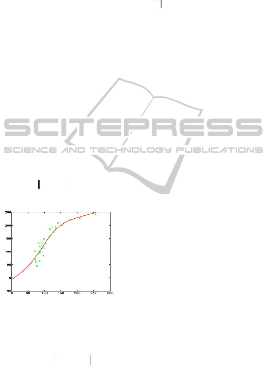
Second, as shown in Fig. 3, an initial SSEs set is

too noisy, and some data points must be dropped. A

classic algorithm for noisy data selection with

dropping outliers is RANSAC algorithm. We use a

slightly modified RANSAC-based scheme:

1) Select a subset of the initial set.

2) Using this subset, estimate cubic smoothing

spline parameters for





according to (26)-(27).

3) For each pair of SSEs, the following

inequality can be computed:



,, ,

tua u

(29)

where t is a threshold. Inequality (29) is true for

inlayer CSEs pairs and false for outliers.

Figure 3: Chromatic shift correction curve for the green

channel, solid points for inlayers CSEs, pitted – for outliers.

After identifying color correction transform

parameters we apply this transform to the image as

the final step of the technique based on model (3)-(4).

To check correction quality we use the following

measure:









max max , ,





px px (30)

where

is Euclidian distance between colors of

corresponding points of two CSEs – source





and corrected





. We know the matching

between the source and the corrected point for color

checker tables. This usually unavailable knowledge

allows us to estimate the value of quality measure

(30), and we will use this measure to evaluate

correction quality.

6 RESULTS

The results of the correction are shown in Fig. 4. The

original picture was captured using a simple, wich

was made as three-step approximation of the Fresnel

lens. First we removed the blur from the green

channel using deconvolution, and then we used edge

analysis for the red and blue channels. Color

correction transform was identified using color

checker table (Fig. 4(c, f)), and finally color

correction was applied to the image.

As shown in Fig. 4, the proposed correction

technique restores both colors and edge information

from distorted images, captured by a simple Fresnel

lens. We compared our color correction technique

with an implementation of Retinex approach from

(Limare et al., 2011). Results for Retinex-based

correction are shown in Fig. 4(e). Visual quality of

color correction exceeds the quality of the Retinex-

based correction. The value of the quality measure

(30) for Retinex is 113 versus 14 for our method.

7 CONCLUSIONS

We show that a simple Fresnel lens can be used for

imaging. Strong aberrations inherent in this optical

system can be restored by digital image processing.

Images captured with a simple Fresnel lens are

corrected with deconvolution and contour analysis

with good results. After we applied deconvolution for

deblurring of the typically less blurred green channel,

we then sharpened the image for other color channels

taking green channel as the guidance image.

After deblurring and sharpening we applied color

correction to remove strong chromatic shift.

Correction transformation was identified using color

checker tables. These tables help to quantify

correction quality, and the proposed correction

technique shows a better quality than the well-known

Retinex method of color correction.

For further research, we see two main directions

ComputationalCorrectionforImagingthroughSingleFresnelLenses

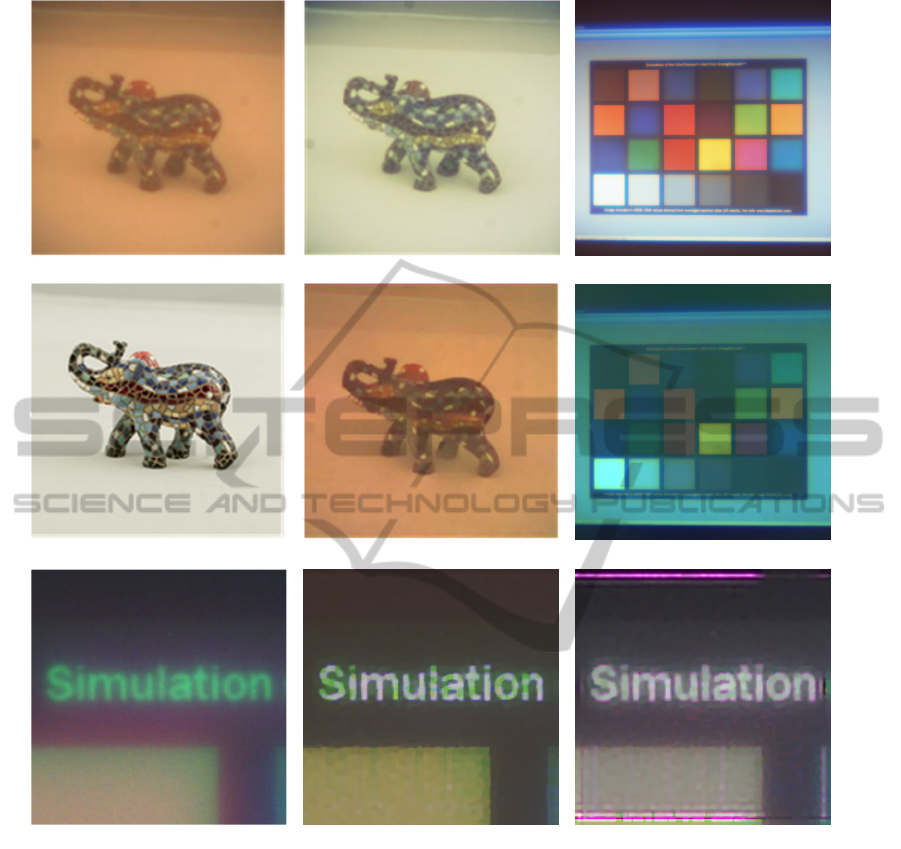
Figure 4: Example of chromatic aberration correction: (a) - image captured by four-step Fresnel lens, (b) - image after color

correction, (d) - image captured by refraction lens, (e) - image after Retinex-based color correction; (c) - color checker image

for correction identification, and (f) - color checker image after correction; (g) - part of color chart, captured by four-step

Fresnel lens, (h) - same part after computational correction, (i) – after final color sharpening.

that may yield additional quality improvements: 1)

increasing the quality of deconvolution, taking into

account the estimation of space-varying PSF and 2)

combining edge analysis and color correction to a

single filter.

ACKNOWLEDGEMENTS

This work was partially supported by project

#RFMEFI57514X0083 by the Ministry of Education

and Science of the Russian Federation.

(a)

(b)

(c)

(d) (e)

(f)

(g) (h)

(i)

SIGMAP2015-InternationalConferenceonSignalProcessingandMultimediaApplications

REFERENCES

Chambolle, A., & Pock, T., 2011. A first-order primal-dual

algorithm for convex problems with applications to

imaging. Journal of Mathematical Imaging and Vision,

vol. 40, no. 1, pp. 120–145.

Cho, T. S., Joshi, N., Zitnick, C. L., Sing Bing Kang,

Szeliski, R., & Freeman, W.T., 2010. A content-aware

image prior IEEE Conference on Computer Vision and

Pattern Recognition, pp. 169-176.

Cho, T. S., Zitnick, C. L., Joshi, N., Sing Bing Kang,

Szeliski, R., & Freeman, W.T., 2012. Image restoration

by matching gradient distributions. IEEE Transactions

on Pattern Analysis and Machine Intelligence, vol. 34,

no. 4, pp. 683-694.

Chung, S.-W., Kim, B.-K., & Song, W.-J., 2010. Removing

chromatic aberration by digital image processing.

Optical Engineering, vol. 49, no. 6, 067002.

Davis, A., & Kuhnlenz, F., 2007. Optical design using

Fresnel lenses - basic principles and some practical

examples. Optik & Photonik, vol. 2, no. 4, pp. 52–55.

Fang, Y. C., Liu, T. K., MacDonald, J., Chou, J. H., Wu, B.

W., Tsai, H. L., & Chang, E. H., 2006. Optimizing

chromatic aberration calibration using a novel genetic

algorithm. Modern Optics, v. 53, no. 10, pp. 1411-1427.

Farrar, N. R., Smith, A. H., Busath, D. R., & Taitano, D.,

2000. In situ measurement of lens aberration. Proc.

SPIE, vol. 4000, March, pp. 18-29.

Gonzalez, R. C., & Woods, R. E., 2001. Digital Image

Processing, Second Edition, Prentice Hall, 2001.

Heide, F., Rouf, M., Hullin, M. B., Labitzke, B., Heidrich,

W., & Kolb, A., 2013. High-quality computational

Imaging Through Simple Lenses. ACM Transactions

on Graphics, vol. 32, no. 5, article No. 149.

Kang, S. B., 2007. Automatic removal of chromatic

aberration from a single image. Computer Vision and

Pattern Recognition, 2007, pp. 1-8.

Limare, N., Petro, A. B., Sbert, C., & Morel, J. M., 2011.

Retinex Poisson equation: a model for color perception.

Image Processing On Line.

Maxwell, B. A., Friedhoff, R. M., & Smith, C. A., 2008. A

bi-illuminant dichromatic reflection model for

understanding images. Computer Vision and Pattern

Recognition, IEEE Conference on, pp. 1–8.

Meyer-Arendt, J. R., 1995. Introduction to Classical and

Modern Optics. Prentice Hall.

Millan, M. S., Oton, J., & Perez-Cabre, E., 2006. Chromatic

compensation of programmable Fresnel lenses. Opics

Express, vol. 14, no. 13, pp. 6226-6242.

Nikonorov, A., Bibikov, S., & Fursov V., 2010. Desktop

supercomputing technology for shadow correction of

color images. Proceedings of the 2010 International

Conference on Signal Processing and Multimedia

Applications (SIGMAP), pp. 124-140.

Nikonorov, A., Bibikov, S., Yakimov, P., & Fursov, V.,

2014. Spectrum shape elements model to correct color

and hyperspectral images. 8th IEEE IAPR Workshop on

Pattern Recognition in Remote Sensing, 2014, pp. 1-4.

Powell, I., 1981. Lenses for correcting chromatic aberration

of the eye. Applied Optics, v. 20, no. 24, pp. 4152–4155.

Shih, Y., Guenter, B., & Joshi N., 2012. Image

enhancement using calibrated lens simulations.

Computer Vision – ECCV 2012, pp. 42-56.

Soifer, V. A. (ed.), 2012. Computer Design of Diffractive

Optics. Woodhead Publishing.

ComputationalCorrectionforImagingthroughSingleFresnelLenses