Optimization of Parallel-DEVS Simulations with Partitioning Techniques

Christopher Herbez

, Eric Ramat

and Gauthier Quesnel

LISIC, ULCO, 50 rue Ferdinand Buisson, 62228 Calais, France

INRA MIAT, 24 chemin de Borde Rouge Auzeville, 31326 Castanet-Tolosan, France

Keywords:

Parallel simulation, Graph partitioning, Parallel-DEVS, Multithreading.

Abstract:

With the emergence of parallel computational infrastructures at low cost, reducing simulation time becomes

again an issue of the research community in modeling and simulation. This paper presents an approach to

improve time of discrete event simulations. For that, the Parallel Discrete EVent System formalism is coupled

to a partitioning method in order to parallelize the graph of models. We will present the graph partitioning

method to realize this cutting and quantify the resulting time savings of parallel implementation. This article

highlights the importance of considering the dynamic of the model when partitioning to improve performances.

Many tests are performed from graphs with different sizes and shapes on several hardware architectures.

1 INTRODUCTION

Modeling complex systems are becoming increas-

ingly costly in time and memory capacity, it is nec-

essary to develop efﬁcient modeling and simulation

tools to address them. DEVS formalism (Zeigler

et al., 2000) and Parallel-DEVS variant (Chow, 1996)

Discrete Event Speciﬁcation is a good candidate to de-

velop a response to both formal and technical. That

i-s a discrete events modeling and simulation the-

ory with a hierarchical approach. The global model,

called structure of the model in DEVS terminology, is

a graph of coupled models. We propose to work from

this models graph to optimize the simulation.

The use of parallel and distributed infrastructure

can make a efﬁcient response of optimization prob-

lem. Our approach is to use a partitioning algorithm

on the graph models in order to parallelize their exe-

cution as efﬁciently as possible.

In (Herbez et al., 2015), we presented this ap-

proach as well as the relative gains obtained for two

types of partitioning. One is based on the connectiv-

ity of the graph, and the other is oriented modeler. In

these examples, the gain obtained by the introduction

of a good partitioning is about 20% compared to an

initial model hierarchy.

The goal of this paper is to show how partitioning

is used to optimize the Parallel-DEVS structure in-

cluding through load balancing between threads and

minimization of exchanges between them. We will

also show the limitations of this approach, and pro-

pose ways to address them. To achieve this, tests are

carried out for two types of graphs and multiple hard-

ware architectures.

In the ﬁrst part, we describe the Parallel-DEVS

formalism and partitioning graph method used for our

tests. Then, various tests on several hardware archi-

tectures will be presented by illustration of the results.

The results will be analyzed to show that it is possible

to evaluate retrospectively the parallel capabilities of

the models. And ﬁnally, a discussion will attempt to

suggest ways to improve the method.

2 FORMALISMS AND METHODS

In this section, the Parallel-DEVS formalism is for-

mally presented and through the main algorithms

for implementation of the formalism. Moreover, we

present the graph partitioning method chose to opti-

mize the Parallel-DEVS simulations.

2.1 Parallel-DEVS

DEVS (Discrete Event Speciﬁcation) (Zeigler et al.,

2000) is a high level formalism based on the discrete

events for the modeling of complex discrete and con-

tinuous systems. The model is a network of intercon-

nections between atomic and coupled models. These

models are in interaction via time-stamped events ex-

changes.

289

Herbez C., Ramat E. and Quesnel G..

Optimization of Parallel-DEVS Simulations with Partitioning Techniques.

DOI: 10.5220/0005543702890296

In Proceedings of the 5th International Conference on Simulation and Modeling Methodologies, Technologies and Applications (SIMULTECH-2015),

pages 289-296

ISBN: 978-989-758-120-5

 2015 SCITEPRESS (Science and Technology Publications, Lda.)

More speciﬁcally, we present the Parallel-DEVS

(PDEVS) formalism (Chow and Zeigler, 1994; Chow,

1996). This extension of the classic DEVS introduces

the concept of simultaneity of events essentially by al-

lowing bags of inputs to the external transition func-

tion. Bags can collect inputs that are built at the same

date, and process their effects in future bags.

PDEVS deﬁnes an atomic model as a set of input

and output ports and a set of state transition functions:

M =

X,Y,S,δ

int

,δ

ext

,δ

con

,λ, ta

With: X, Y, S are respectively the set of input values,

output values and sequential states

ta : S → R

is the time advance function

int

: S → S is the internal transition function

ext

: Q ×X

→ S is the external transition function

where:

Q = {(s,e)|s ∈ S,0 ≤ e ≤ ta(s)}

Q is the set of total states,

e is the time elapsed since last transition

is a set of bags over elements in X

con

: S × X

→ S is the conﬂuent transition

function, subject to δ

con

(s,

0) = δ

int

(s)

λ : S → Y is the output function

If no external event occurs, the system will stay

in state s for ta(s) time. When e = ta(s), the system

changes to the state δ

int

. If an external event, of value

x, occurs when the system is in the state (s, e), the

system changes its state by calling δ

ext

(s,e,x). If it

occurs when e = ta(s), the system changes its state

by calling δ

con

(s,x).

Every atomic model can be coupled with one or

several other atomic models to build a coupled model.

This operation can be repeated to form a hierarchy of

coupled models. A coupled model is deﬁned by:

N = hX,Y,D,{M

},{I

},{Z

i,d

Where X and Y are input and output ports, D the

set of models and:

∀d ∈ D,M

is a PDEVS model

∀d ∈ D ∪ {N}, I

is the inﬂuencer set of d :

⊆ D ∪{N}, d /∈ I

,∀d ∈ D ∪ {N},

∀i ∈ I

i,d

is a function,

the i-to-d output translation:

i,d

: X → X

, if i = N

i,d

: Y

→ Y, if d = N

i,d

: Y

→ X

, if i 6= N and d 6= N

The inﬂuencer set of d is the set of models that

interact with d and Z

i,d

speciﬁes the types of relations

between models i and d.

PDEVS is an operational formalism. This means

that the formalism is executable and thus it provides

algorithms for its execution. These algorithms deﬁne

the sequence of the different functions of the PDEVS

structure. Moreover, the atomic and coupled models

are respectively associated with simulators and co-

ordinators. The aim of simulators is to compute the

various functions while the coordinators manage the

synchronization of exchanges between simulators (or

coordinators in a hierarchical view).

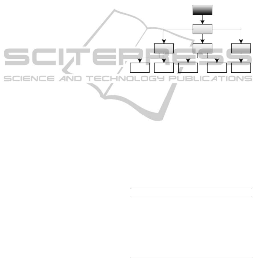
Figure 1: Hierarchy of coordinators and simulators. Black

box is the root coordinator (manage simulation), Grey boxes

are coordinators (simulate coupled models) and white boxes

are simulators (simulate atomic models).

2.2 PDEVS Algorithms

In this article, we explain the PDEVS abstract sim-

ulators especially the algorithms of the coordinator

which allows concurrent simulation between the com-

ponents of the coordinator. Indeed, the Parallel-

DEVS approach to parallelize simulation uses a risk-

free and strict causality adherence. It uses a global

minimum time synchronization and allows a concur-

rent and simultaneous output collection and distribu-

tion of events

Algorithm 1: Parallel-DEVS-Coordinator.

1: procedure VARIABLES

2: DEV S = (X ,Y,D,{M

},{i

},{Z

i,d

})

3: parent: parent coordinator

4: tl, tn

5: event − list: list of elements (d,tn

) sorted

6: IMM: imminent children

7: mail: output mail bag

8: y

parent

9: {y

}

In Figure 1, coordinator are represented by the

grey boxes. Each coordinator manages a scheduler

and route messages between children. The scheduler

stores internal events (one internal event per child)

SIMULTECH2015-5thInternationalConferenceonSimulationandModelingMethodologies,Technologiesand

Applications

290

sorted by time to wake up models. These times are

produced using the ta function for atomic models and

the current date of the simulation. For each itera-

tion, coordinator build a set of immediate message (all

events with the same wake up time).

Algorithm 2: Parallel-DEVS-Coordinator.

1: procedure WHEN RECEIVE I-MESSAGE(i, t) AT

TIME t

2: for each d ∈ D do

3: send i-message to child d in parallel way

4: sort event-list according to tn

5: tl = max{tl

|d ∈ D}

6: tn = min{tn

|d ∈ D}

Algorithm 3: Parallel-DEVS-Coordinator.

1: procedure WHEN RECEIVE *-MESSAGE(∗, t)

2: if t 6= tn then

3: error: bad synchronization

4: IMM = {d|(d,tn

) ∈ (event-list ∧tn

= tn)}

5: for each r ∈ IMM do

6: send *-message (*, t) to r in parallel way

Algorithm 4: Parallel-DEVS-Coordinator.

1: procedure WHEN RECEIVE X-MESSAGE(x, t)

2: if ¬(tl 6 t 6 tn) then

3: error: bad synchronization

4: receivers = {r|r ∈ D, N ∈ I

N,r

(x) 6=

5: for each r ∈ receivers do

6: send x-message (Z

N,r

(x), t) to r in parallel

way

7: for each r ∈ IMM ∧ ¬ ∈ receivers do

8: send x-message (

0, t) to r in parallel way

9: sort event-list according to tn

10: tl = t

11: tn = min{tn

|d ∈ D}

Messages received by a coordinator are described

in the algorithms 1, 2, 3, 4 and 5. i-message is used

to initialize children. *-message is used to compute

output of children. x-message and y-message are

used to route messages. In PDEVS, all imminents

(IMM) are allowed to execute concurrently in con-

trast to DEVS where imminents were sequentially ac-

tivated. The outputs of IMM are collected into a bag

called the mail in previous algorithms. The mail is an-

alyzed for the part going out because of the EOC and

the parts to be distributed internally to the components

due to the IC coupling. The internal transition func-

tions of the imminents are not executed immediately

since the may also receive input at the same model

time.

Algorithm 5: Parallel-DEVS-Coordinator.

1: procedure WHEN RECEIVE Y-MESSAGE(y

, t)

WITH OUTPUT y

FROM d

2: if this is not the last d in IMM then

3: add (y

, d) to mail

4: mark d as reporting

5: else

6: if this is the last d ∈ IMM then

7: y

parent

8: for each d ∈ I

∧ d is reporting do

9: if Z

d,N

) 6=

0 then

10: add y

to y

parent

11: send y-message(y

parent

, t) to parent

12: for each child r with some d ∈ I

∧d is report-

ing ∧Z

d,r

) 6=

0 do

13: for each d ∈ I

∧ d is reporting

∧Z

d,r

) 6=

0 do

14: add Z

d,r

) to y

15: send x-message(y

,t) to r

16: for each r ∈ IMM ∧ y

0 do

17: send x-message(

0,t) to r

18: sort event-list according to tn

19: tl = t

20: tn = min{tn

|d ∈ D}

2.3 Graph Partitioning and Parallel

Mode

Using graph partitioning to transform the model hier-

archy in another in order to be optimized for parallel

simulations, this work is possible thanks to the clo-

sure under coupling property of DEVS (Zeigler et al.,

2000). This property formally describes the coupled

model is equivalent to an atomic model. Thus an

atomic model can be move into a new coupled model

and all the hierarchy of coupled model can be merge

into a unique coupled model.

The result of the coupled model hierarchy merge

give an oriented graph. In mathematics, a graph is de-

ﬁned by G = (V, E) where V is the vertices set and

E the edges set. For the simulation, V describe the

atomic models and E the connection network between

them. Moreover, a weight could be associated to each

vertex and edge. For vertices, the weight quantify the

execution time and for edges quantify the data propor-

tion transmitted between models. Slower is a model,

bigger is his weight.

The k-way graph partitioning allows to cut a graph

G into k subgraphs {G

,. .. ,G

}, while minimiz-

OptimizationofParallel-DEVSSimulationswithPartitioningTechniques

291

ing one or more criterion. They are represented by

functions named “objective function”. This cutting

provides k subsets of vertices P

= {V

,. .. ,V

} ⊂

V named partition. Each vertex of a part V

is executed

on the same simulation node or logical process (LP).

For reduce the simulation time, it’s necessary equal-

ize the execution time on each LP and minimize the

events exchange between them. This can be reﬂected

by the partition quality. To be good quality, a parti-

tion must respect some conditions: the parts weight

must be similar and connections between parts must

be minimal.

The objectives of our research are to reduce execu-

tion time for very large simulations (more than 20000

models). These simulations give very large model

graphs. It is necessary to use partitioning graph meth-

ods efﬁcient for this graph size. We use a multilevel

scheme in order to solve the problem.

The following subsection present the objective

functions used for partitioning in order to minimize

the simulation time.

2.3.1 The Objective Function

The partition quality is given by the objective func-

tions. Smaller is the result, better is the partition qual-

ity. They revolve around two concepts: cost cutting

between partition parts and parts weight.

Given a partition P

= {V

,...,V

}, the edge cut

of two parts is the weight sum of edges connecting V

and V

Cut(V

) =

∑

∈V

weight(v1,v2) (1)

For a partition P

, the edge cut is the weight sum

of edges connecting partition parts:

Cut(P

) =

∑

i< j

Cut(V

) (2)

This objective function was already used by Brian

Kernighan and Shen Lin in (Kernighan and Lin,

1970).

Another function allows simultaneous manage-

ment the minimization of the edge cut and weight bal-

ance between parts: the ratio cut:

Ratio(P

) =

∑

i=1

Cut(V

,V −V

)

weight(V

)

(3)

It was introduced by Yen-Chuen Wei and Chung-

Kuan Cheng in (Wei and Cheng, 1989). In our works,

we seek to minimize this objective function.

2.3.2 The Multilevel Method

As introduce in (Herbez et al., 2015), we used a mul-

tilevel schemes to create quickly a graph partition of

big size. It consists of three phases:

• Coarsening: Graph reduction by successive ver-

tices matching, while keeping the nature of the

original graph. Iterative process generating a

graph base {G

,· ·· ,G

}, where G

= G the origi-

nal graph and G

the contracted graph. The Heavy

Edge Matching introduced in (Karypis and Ku-

mar, 1998) is implemented for this phase.

• Partitioning: Creating of a partition P

of the

coarsening graph G

using a partitioning heuris-

tic. We choose an expanding region method: the

Greedy Graph Growing Partitioning (Karypis and

Kumar, 1998).

• Uncoarsening: Projection of the partition P

each contraction graph levels G

(i = n − 1,...,1).

But after each projection it is necessary to realize

a reﬁnement for keep a good quality. We use a

local optimization algorithm based on Kernighan-

Lin algorithm (Kernighan and Lin, 1970)

For convenience, the multilevel implementation

using GGGP as partitioning phase will be call GGGP.

3 DATA, SOFTWARE AND

HARDWARE

This section presents the data on which the tests were

conducted, as well as the different used hardware ar-

chitectures.

3.1 Data Description

Tests were realized from two classical graph types in-

spired by the water ﬂow model: a grid and a “tree”

(abusively named). We have choose these names be-

cause they reﬂect the graph form, even if in the liter-

ature a “tree graph” is a hierarchical graph. It’ is not

the case here. For each graph, the vertices weight is

equal to 1 because the execution time of the models

is the same. The edge weight is equal to 1 because

the message transfer cost is the same between each

model. We work on large simulations, where graphs

have 20000 vertices. They are presented in Figure 2.

The left graph consists of several levels, where

there are a single vertex source and outlet. The ver-

tex source is the starting model of the simulation and

the outlet is the ending model. Each vertex of level n

is connected with two vertices of level n − 1. For the

SIMULTECH2015-5thInternationalConferenceonSimulationandModelingMethodologies,Technologiesand

Applications

292

penultimate level, vertices are connected only to the

outlet.

Figure 2: Little graphs size examples. On the left, a “grid

graph” and on the right a “tree graph” (abusively named).

The right graph is composed of several branches,

where each vertex is connected to one or more ver-

tices following a single direction. The branches are

branched until reaching the single outlet. This graph

have several source vertices on each top branch (n

sources by branches).

3.2 Software and Hardware

Architectures

The tests were performed on a PDEVS simula-

tion kernel written in C++11. This simulation ker-

nel is part of the VLE project (Virtual Laboratory

Environment) a modeling and simulation software

suite (Quesnel et al., 2009). The VLE software suite

is used in many projects in the French National In-

stitute for Agronomical Research and several French

Universities.

The simulations were done on an three different

hardware architectures:

• Intel Core i5-2520M processor - 2.5 GHz: 2 cores

with 4 threads (hyperthreading mode)

• Intel Core i7-3840QM processor - 2.8 GHz: 4

cores with 8 threads (hyperthreading mode)

• Samsung Exynos 5422 with a Cortex A15 2.1 Ghz

quad core and a Cortex A7 1.5 GHz quad core

processor: 4 big cores and 4 little cores

These four used architectures to test different al-

gorithms on architectures with different possibilities

in terms of cores. The smallest conﬁguration allows

to have two cores with a small speedup factor of four

threads (2C + 2H). The second doubles possibilities

(4C + 4H). The third offers a hybrid solution (4C +

4LC) slightly greater than the second.

4 RESULTS AND DISCUSSION

In this section, we present simulation results on clas-

sical models which we employ in our scope (nitrogen

and water management in catchment area). For that,

PDEVS formalism and the partitioning algorithm, in-

troduced in section 2, are used on several hardware

architectures.

The results are then discussed to evaluated the

performance and limitations of our approach. These

tests are performed from the graphs presented in Sec-

tion 3.1.

4.1 Results Analysis

The simulation results presented in this subsection are

obtained for a computation time of about 1 ms by

models. Our goal is to compare the performance ob-

tained with those expected in theory.

In absolute terms, the expected performance for

parallelization tend to have a speedup equal to the

available thread number. It is named absolute theo-

retical speedup. However, given the dynamic of the

models, it is very difﬁcult to achieve this performance

in pessimistic approach. In order to have an effective

comparison basis, we propose to compute a theoreti-

cal speedup including the dynamics of the models.

The following subsection present this theoretical

speedup and an illustration to explain its operation.

4.1.1 Theoretical Speedup Deﬁnition

For a given transition, the theoretical speedup is de-

ﬁned by the ratio of the sum of active atomic models

and the maximum number of active models in one of

the coordinators. This is expressed mathematically

by:

Speedup =

∑

i=1

max

i∈{1,...,k}

(4)

where k is the coordinator number and n

the active

models number in the coordinator i.

The active models are the models included in the

IMM set when the transition function is executed.

The active models in a same coordinator form a bag.

For a given date, the bags size varies according to

the event propagation in the global model. If the bag

size is the same then the theoretical speedup is equal

to the number of active coordinators (since there is

OptimizationofParallel-DEVSSimulationswithPartitioningTechniques

293

one thread per coordinator and that, depending on the

hardware architecture, all threads can be executed in

parallel modulo the memory access). This concept is

illustrated in Figure 3.

inf

T = t

Time step

inf

Part 1

Part 2

Schedulers

Root

C1 C2

inf

t+1

inf

t+1

inf

T = t

T = t+1

inf

t+1

inf

C1 C2

DEVS hierarchy

Caption

Active models

(bags)

Figure 3: Illustration of the schedulers evolution for a time

step on a small example.

This diagram shows different information from a

simulation at time t. The sub-diagram at top show a

graph models partitioned in two parts. His hierarchi-

cal representation is given at bottom on the left. Each

coordinator has a scheduler. Their evolution, for each

transition, is shown at the bottom right. Active mod-

els are represented by the shaded boxes. All active

models of a same coordinator form a bag. For the

ﬁrst transition (M

) and (M

) form two bags, so

the speedup of this transition is 1.5. The speedup is

computed for each transition. Here, there are 3 tran-

sitions with a respective speedup 1.5, 2 and 1.

For a give date t, n

-speedup are computed (n

the transition number). Figures 6 et 7 show this vari-

ation at the date t = 0. The theoretical speedup of a

date t is the mean of speedups at each transition:

Speedup(t) = mean(Speedup) (5)

And the speedup of the simulation is:

Theoretical

Speedup = mean(Speedup(t)) (6)

This theoretical speedup is closely linked to the

hierarchy of coordinators / simulators. It is important

to create balanced sub-models. But this is not enough,

it is necessary to have a balance between bags at each

transition to ensure a perfect balance. In our case, all

models have the same charge in terms of calculation,

that’s why we talk about model number and not model

weight.

4.1.2 Inﬂuence of the Hardware Architecture on

Speedup

Figures 4 and 5 compare the evolution of the speedup

for different hardware architectures to the theoretical

speedup. For that, we vary the number of threads (par-

tition number) and we observe the impact on the evo-

lution of the speedup.

Figure 4: Speedup for tree graphs with 3 hardware architec-

tures and theoretical speedup.

Figure 5: Speedup for grid graphs with 2 hardware archi-

tectures and theoretical speedup.

These curves show the inﬂuence of the hardware

architecture on the speedup. Indeed, until the number

of threads is less than or equal to the number of cores,

the speedup is very close to the theoretical value. For

architecture 4C + 4LC, a slight inﬂection is observed

with 8 threads because the 4 additional cores are less

efﬁcient than the ﬁrst 4 cores.

4.1.3 Link between Theoretical Speedup and

Partitioning Quality

The results presented in this subsection are obtained

from graph of size 1000 and a hierarchical structure

with four sub-models. The theoretical speedup can be

a partition quality indicator, as shows this subsection.

In the Figure 6, the transition function is com-

puted 63 times where 1/3 of them the number of ac-

tive sub-models is equal to 1. So the parallelization is

not used during this phase. By against, the remaining

two thirds show a efﬁciency close to the optimum (4).

Given the graphs structure, it is hard to beat.

For the grid (Figure 7), the conclusion is not the

same. We are far to the absolute theoretical speedup

with 4 threads (max = 2.2). This is explained by the

dynamics of the grid model: the events propagate by

SIMULTECH2015-5thInternationalConferenceonSimulationandModelingMethodologies,Technologiesand

Applications

294

Figure 6: Variation of theoretical speedup at t = 0 for “tree”.

wave from the top left corner to the bottom right cor-

ner. For the partitioning, the grid is divided in 4 al-

most regular sub-grids. The number of models com-

puted in parallel can be at most 2 (or 3 in some limit

cases).

Figure 7: Variation of theoretical speedup at t = 0 for

“grid”.

Figure 7 suggests that partitioning is not optimal

in this case. It does not take sufﬁcient account of the

dynamics of the model. However, the particular struc-

ture of this graph does that the theoretical speedup can

not always be equal to the absolute because the num-

ber of parallelizable models is lower than the number

of threads available at times. This is particularly the

case in the beginning and end of the simulation.

Figure 8: Speedup of gggp and random method on ”grid”.

To be convinced of the phenomenon, we generate

a random cutting and compare the theoretical speedup

that obtained with our partitioning method. Figure 8

shows that the random cutting has a greater theoretical

speedup for a parts number less than 8.

4.2 Results Discussion

The results show that in one case (tree), our partition-

ing method leads to the construction of a hierarchy

similar to the optimum of the theoretical speedup per-

spective. The second case (grid), the results are not

up to par. In fact, there are more suitable cuts which

follow the dynamics of the model. The optimal cut-

ting is computable and depends on the graph structure

and of the dynamics of the model. For each bag, di-

viding the cardinality of the IMM set by the number

of coordinators, we take the integer part. If the mod-

ulus of the two terms is not zero then added one (see

7). We then obtain the optimal size of bags that are

processed by each coordinator. The average is then

carried out on all the transitions (2N − 1 transitions

for a grid size N) for a time step. We obtain then

the theoretical speedup in optimum for the grid. The

equation of optimal speedup in this case is:

S bag(k) = b

c + hk mod Pi (7)

Speedup = mean(2

N−1

∑

i=1

S bag(i) + S bag(N)) (8)

We can then compare the theoretical speedup of

our partitioning compared to the theoretical speedup

of the best partitioning (see Figure 9).

Figure 9: Speedup comparison to the absolute for a ”grid”.

The objective of partitioning is to obtain a speedup

equal to the number of cores provided on the machine

during almost all of the simulation. To be a good

quality, the partition shall enable at the results to be

close to this speedup. Which is not actually our case

here. The partitioning method must not only balance

the loads among threads, it must also take into ac-

count the dynamics of the graph. The knowledge of

the dynamics minimizes the load difference between

OptimizationofParallel-DEVSSimulationswithPartitioningTechniques

295

the bags at each transition. This allows better man-

agement of threads throughout the simulation.

If the models were fully synchronous as in the

case of a cellular automaton, the issue of balanc-

ing would be easy to solve if all models have the

same computational load. In this case, we observe

no change in the number of transitions to be made be-

tween two time steps. The partitioning becomes use-

less. In contrast, if the models are completely asyn-

chronous, the IMM sets have a single model. Paral-

lelization is completely useless in a pessimistic con-

text. In this case, it was essential to work on algo-

rithms optimistic parallel simulation.

5 CONCLUSION AND

PROSPECTS

In this paper, we have shown that in some cases,

we improve the simulation time by using a partition-

ing based solely on the model structure. These sim-

ulations are performed using an implementation of

PDEVS algorithms in a risk-free mode. However, we

have shown that it is also necessary to consider the

dynamic of models for have a better models balance.

We have shown that the measure of the theoretical

speedup (see equation 4) based on the IMM set gives

us accurate information. We can generalize this mea-

sure so that it becomes an parallelization ability indi-

cator of a model. This indicator can vary from 1 to P

where P is the parts number of the graph. The mini-

mum value is obtained for fully asynchronous model

and the maximum value for fully synchronous model.

In our case, the indicator takes values close to the

maximum value. This means that a coupling between

a partitioning method and risk-free simulation is an

excellent approach. However, it is necessary to go fur-

ther if the indicator is close to 1. May be introduce a

conservative or optimistic simulation engine coupled

with partitioning methods. The model structure must

be consider, but also his dynamics and the conser-

vative algorithms with look-head properties (Chandy

and Misra, 1979; Chandy and Misra, 1981) or opti-

mistic (Time-Wrap (Jefferson, 1985), for example).

Look-head is the ability of a model to predict that it

will not have output for a certain period in future. The

complexity of the optimization algorithm will be in-

creased. It will be necessary to understand the interac-

tions between look-head, for example, dynamics and

the models graph.

Furthermore, our strategy of optimized hierarchy

building has the overall objective to integrate dis-

tributed hardware architecture where the communica-

tion time between processes are not negligible.

ACKNOWLEDGEMENTS

This work is carried out in research project named Es-

capade (Assessing scenarios on the nitrogen cascade

in rural landscapes and territorial modeling - ANR-

12-AGRO-0003) funded by French National Agency

for Research (ANR).

REFERENCES

Chandy, K. M. and Misra, J. (1979). Distributed simulation:

A case study in design and veriﬁcation of distributed

programs. IEEE Trans. Software Eng., 5(5):440–452.

Chandy, K. M. and Misra, J. (1981). Asynchronous dis-

tributed simulation via a sequence of parallel compu-

tations. Commun. ACM, 24(4):198–206.

Chow, A. C.-H. (1996). Parallel devs: A parallel, hierarchi-

cal, modular modeling formalism and its distributed

simulator. Trans. Soc. Comput. Simul. Int., 13(2):55–

67.

Chow, A. C. H. and Zeigler, B. P. (1994). Parallel devs: A

parallel, hierarchical, modular, modeling formalism.

In Proceedings of the 26th Conference on Winter Sim-

ulation, WSC ’94, pages 716–722, San Diego, CA,

USA. Society for Computer Simulation International.

Herbez, C., Quesnel, G., and Ramat, E. (2015). Building

partitioning graphs in parallel-devs context for paral-

lel simulations. In Proceedings of the 2015 Spring

Simulation Conference.

Jefferson, D. R. (1985). Virtual time. ACM Trans. Program.

Lang. Syst., 7(3):404–425.

Karypis, G. and Kumar, V. (1998). A fast and high qual-

ity multilevel scheme for partitioning irregular graphs.

SIAM J. Sci. Comput., 20(1):359–392.

Kernighan, B. W. and Lin, S. (1970). An efﬁcient heuristic

procedure for partitioning graphs. Bell System Techni-

cal Journal, 49(2):291–307.

Quesnel, G., Duboz, R., and Ramat, E. (2009). The Virtual

Laboratory Environment – An operational framework

for multi-modelling, simulation and analysis of com-

plex dynamical systems. Simulation Modelling Prac-

tice and Theory, 17:641–653.

Wei, Y.-C. and Cheng, C.-K. (1989). Towards efﬁcient

hierarchical designs by ratio cut partitioning. In

Computer-Aided Design, 1989. ICCAD-89. Digest of

Technical Papers., 1989 IEEE International Confer-

ence on, pages 298–301.

Zeigler, B. P., Kim, D., and Praehofer, H. (2000). Theory of

modeling and simulation: Integrating Discrete Event

and Continuous Complex Dynamic Systems. Aca-

demic Press, 2nd edition.

SIMULTECH2015-5thInternationalConferenceonSimulationandModelingMethodologies,Technologiesand

Applications

296