
Nonlinear System Identification based on Modified ANFIS
Jos
´
e Kleiton Ewerton da Costa Martins and F
´
abio Meneghetti Ugulino de Ara
´
ujo
Universidade Federal do Rio Grande do Norte,
Departamento de Engenharia da Computac¸
˜
ao e Automac¸
˜
ao (DCA),
Natal, Rio Grande do Norte, Brazil
Keywords:
ANFIS, Modified ANFIS, Nonlinear Systems Identification, Linear Systems Identification.
Abstract:
This article aims to present the nonlinear system identification by the method of modified ANFIS. The modi-
fied ANFIS is a structure proposed that is based on the traditional structure of ANFIS with some modifications
as shown in the article. The importance of the choice of method parameters and its influence on the system will
be discussed. For this, the identification of a coupled system of tanks with nonlinear dynamics is performed.
System identification will be performed by changing the inputs and order of the consequent model and then
will perform a review of the systems. The results confirm the simplicity of modified ANFIS in comparison
with the traditional ANFIS while have good performance in the identification of nonlinear systems.
1 INTRODUCTION
To have a thorough knowledge of a system is nec-
essary to examine, analyze and simulate a system of
interest. Linear systems identification techniques are
used since 1960 to those needs.
Linear models are widely used in different areas
of knowledge. In general, this type of model is ap-
plied to a specific region known as operating point,
which is necessary to make a linearization can use the
model. This is necessary because most real systems
are nonlinear. Industry plants are complex systems
and most of them are nonlinear. Due to this nonlinear-
ity, the identification of nonlinear systems is becom-
ing a very important tool which is used to improve the
performance of a controller, prevent the modeling of
the phenomenological model and obtain a nonlinear
model whitch previoles a representation more similar
to the system response.
The identification of nonlinear systems is be-
ing largely performed by Artificial Intelligence tech-
niques. The fuzzy systems and Artificial Neural Net-
works (ANNs) are the most used techniques.
The ANN has characteristics that make it attrac-
tive for use in applications such as the identification of
nonlinear dynamical systems, such as the generaliza-
tion ability and learning. According (Haykin, 2001),
it is clear that a neural network draws its computing
power through first, its massively parallel distributed
structure, and second, their ability to learn and there-
fore generalize. The spread refers to the fact that
the neural network produce appropriate outputs to in-
puts that were not present during training (learning).
These two information processing capabilities make
it possible for the neural networks solving complex
problems (large scale) that are currently untreatable.
The ANN has disadvantages including the appro-
priate choice of structured network, ie, how many lay-
ers, how many neurons in each layer must have the
neural network, find out what activation function of
neurons in each layer, may become an arduous and
exhausting work.
Among the different nonlinear identification tech-
niques, methods based on neuro-fuzzy models are
gradually becoming established, not only in the
academia but also in industrial applications. Neuro-
fuzzy systems combine the semantic transparency of
rule-based Fuzzy systems with the learning capability
of Neural Networks. Both neural networks and fuzzy
systems are motivated by imitating human reasoning
processes. Fuzzy systems, relationships are repre-
sented explicitly by if-then rules. In neural networks,
the relations are not explicitly given, but are ’coded’
in the network and its parameters. In contrast to
knowledge-based techniques, no explicit knowledge
is needed for the application of neural nets (Babuka,
2003).
The most used neuro-fuzzy nonlinear system iden-
tification process is the Adaptive Neuro-Fuzzy Infer-
ence Systems (ANFIS) developed by (Jang, 1993).
The significance of ANFIS model is, firstly build
588
Ewerton da Costa Martins J. and Araújo F..
Nonlinear System Identification based on Modified ANFIS.
DOI: 10.5220/0005544905880595
In Proceedings of the 12th International Conference on Informatics in Control, Automation and Robotics (ICINCO-2015), pages 588-595
ISBN: 978-989-758-122-9
Copyright
c
2015 SCITEPRESS (Science and Technology Publications, Lda.)

identification form of nonlinear system is not re-
quired, provided that ANFIS is an identification form
itself. Its network weight value consists of adjustable
parameters. This system can identify nonlinear sys-
tems in temperament and in result the network can
approach the input and output data of the system. AN-
FIS gather the advantages of both fuzzy identifica-
tion and neural network identification. It takes lesser
computational epochs than neural network for highly
real nonlinear systems. It contracts with the structure
knowledge with weaken speed and strong submerge.
ANFIS can also be used to control online system fore-
cast systems output instead of real physical systems
(ZhixiangHow, 2003).
An alternative to the identification of nonlinear
systems is modified ANFIS method proposed by
(Fonseca, 2012). This has obtained by modification
of the ANFIS proposed by (Jang, 1993). The identi-
fication of nonlinear systems using the modified AN-
FIS is performed through the local linear models iden-
tified and subsequently trained by backpropagation
training algorithm, and performing the combination
of these local models for a nonlinear system identi-
fication which fully represents the plant. The modi-
fied ANFIS also has some advantages over the origi-
nal ANFIS, as will be showing in the case study.
In this paper we present a case study where was
identified 6 models using the modified ANFIS, chang-
ing the order of local models and the auxiliary vari-
able. An order analysis of the local models was per-
formed as well as the quantity and the importance
of the auxiliary variable in the modified ANFIS. For
the case study was using a didactic plant Quaser with
nonlinear dynamics to perform the identification of
system.
The next sections of this paper is organized as fol-
lows. Section 2 will present the main theoretical con-
cepts necessary for the work development. Section
3 will present an application of the modified ANFIS.
Section 4 will present the main results and contribu-
tions made by the development of this work.
2 THEORICAL
FUNDAMENTATION
Adaptive Neuro-Fuzzy Inference Systems (ANFIS)
developed by Jang (Jang, 1993), can be seen as an
artificial neural network of six layers interconnected
by individual weights, where each layer is responsi-
ble for an operation result in output equivalent to that
found in a particular stage of a fuzzy system Takagi-
Sugeno (Jang, 1993) (Jang and Sun, 1995).It is there-
fore an hybrid technique, Artificial Intelligence that
infers knowledge using the principles of fuzzy logic to
this structure and adds the possibility of the inherent
learning ANN. One of the main advantages of AN-
FIS in relation to ANN is the way of encoding knowl-
edge. While this one is encoded in weights, whose ac-
tions are difficult to interpret, the ANFIS knowledge
is encoded in a structure that has a certain approach
of logic used by humans.
2.1 Hybrid Learning Algorithm
This algorithm has been proposed with the ANFIS
is a hybrid algorithm which combines the gradient
method and the least squares estimate (LSE) to iden-
tify parameters. More specifically, in the forward pass
of the hybrid learning algorithm, functional signals go
forward till layer 4 and the consequent parametrs are
identified by the least squares estimate. In the back-
ward pass, the erro rates propagate backward and the
premise parameters are updated by the gradient de-
scent (Jang, 1993).
2.2 Backpropagation in ANFIS Model
In backpropagation algorithm is necessary to have the
error estimation, the difference of the desired value
and output the estimated model, so that through gra-
dient descent is made to update the parameters. In
ANFIS the estimation error is calculated through the
layer 5 and so propagated to the previous layers, as
can see in (Jang, 1993).
2.3 The Modified ANFIS
The modified ANFIS proposed by (Fonseca, 2012),
is a modification of ANFIS to obtain a system-
atic method for identifying, from linear identification
techniques. This method gets local linear models and
are combined by the modified ANFIS structure. Af-
ter the modified ANFIS training is obtained a global
identification of the plant.
The modification made to the ANFIS consists of
independently leaving the inputs of the first and fifth
layers, ie, may be the same or not, depending on the
purpose and desired accuracy for the application. This
method is divided into four steps.
The first step consists in dividing the plant uni-
verse of discourse in operating points, around which
can be obtained linear models representing operating
regions. It should be chosen the least number of pos-
sible operating points, able to satisfactorily represent
the plant throughout the operating range. This way,
you avoid the unnecessary increase in complexity and
computational cost.
NonlinearSystemIdentificationbasedonModifiedANFIS
589
In the second step, it is performed the identifica-
tion and validation of linear models around the oper-
ating points chosen in second step. Therefore, in this
step, are obtained the local models. These models are
used as consequent of the rules of the modified AN-
FIS.
Next, in step three, is made the training of the
modified ANFIS, determining a way the models iden-
tified in the previous step should be combined to
reproduce adequately the nonlinear behavior of the
plant throughout its universe of discourse.
Finally, the last step is made the validation, which
checks the modified ANFIS capacity to give a re-
sponse that is approximately equal to the plant to a
different input those presented in the training.
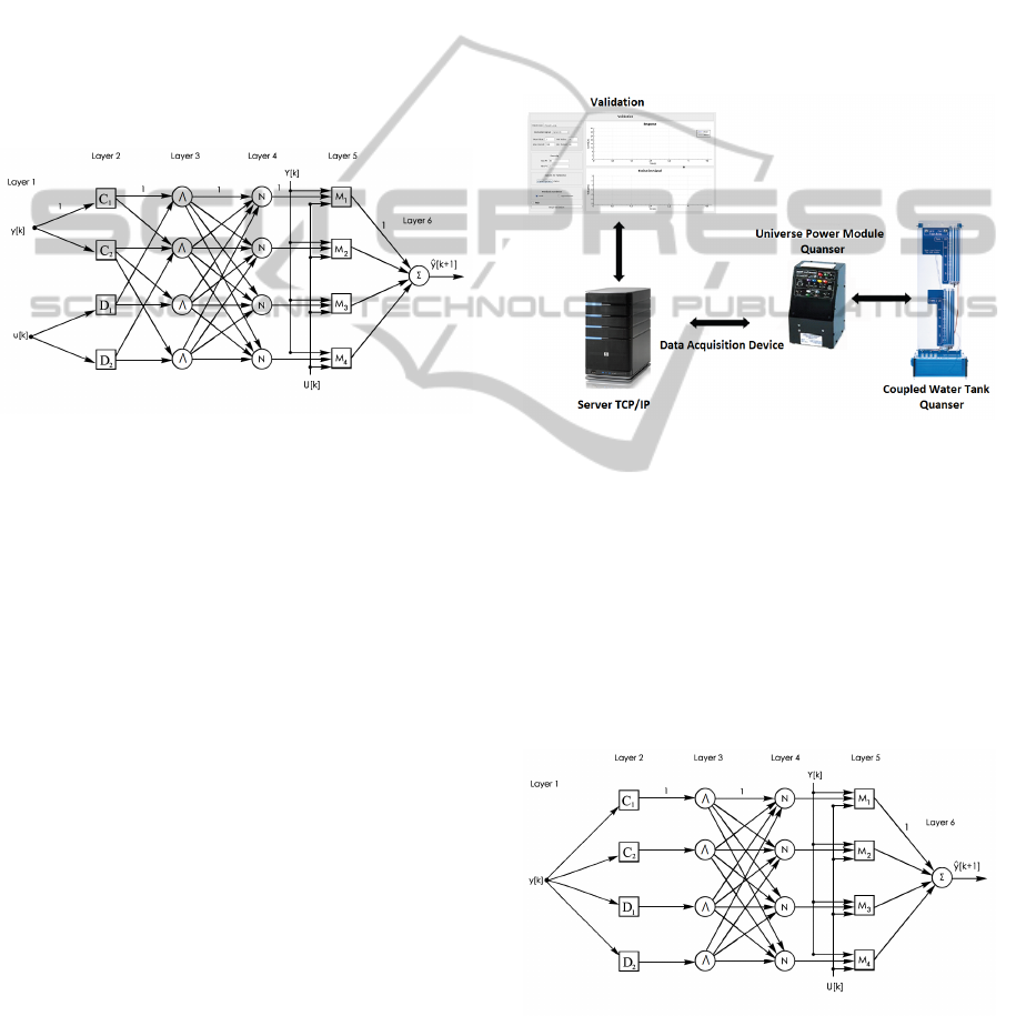
Figure 1: ANFIS modified example of the structure.
The neuro-fuzzy structure illustrated in Figure 1
presents: two inputs, which are the plant output at
the current time point y(k) and the input signal ap-
plied to the plant at the current time u(k); two mem-
bership functions for each input variable, resulting in
four rules; and a linear model designed for the conclu-
sion of each rule, i.e, for each operating point, which
in the illustrated case is four. It can be seen that lin-
ear models for this case are functions of the output
vector Y(k) and input U(k) of the plant. Such vec-
tors may contain current and previous values, or just
the current values, making equal the inputs of iden-
tifiers and the ANFIS, allowing the ANFIS structure
is maintained, since the models are functions of their
inputs (Fonseca, 2012).
3 CASE STUDY
The chosen case study was a system of tanks coupled
with nonlinear dynamics. They were a Quanser di-
dact plant (Apkarian, 1999), consisting of two cou-
pled tanks, also containing a pump and a reservoir.
The two tanks contain a hole in its base, which allows
the flow of water. The upper tank receive the pumped
water from the reservoir, making it the top tank feeds
the lower tank through the hole at its base and the
lower tank closes a cycle with the water back to the
reservoir at its orifice. The tanks have a height of 30
cm, so the liquid level can vary in a range of 0 to 30
cm. The pump receives a voltage which can vary in
the range of 0 to 4 volts, makes the pump pumping
the liquid to the tanks. In Figure 2, we can see a rep-
resentation of the coupled tank system, as well as the
schematic plan of communication. The communica-
tion software developed to plan is made via a TCP / IP
server which is connected to a data acquisition board,
making it possible to read the sensors and writing an
electrical signal to the pump.
Figure 2: Comunication between software and the system.
The analysis of this case study allows an evalu-
ation of the structure modified ANFIS, exploring its
flexibility in a plant with non-linearity. Thus, the sys-
tem described identification was made using the mod-
ified ANFIS. We identified six global models varying
the order of local models and the auxiliary variable
used in the modified ANFIS input(layer 1).The appro-
priate choice of local models and the auxiliary vari-
able directly influence the modified ANFIS structure
as can be seen in the figure 3.
Figure 3: Structure ANFIS modified with an input.
As can be seen in Figure 3,from the structure of
the modified ANFIS, a change in local order model
will change the number of elements of the vector Y(k)
ICINCO2015-12thInternationalConferenceonInformaticsinControl,AutomationandRobotics
590

and U(k). For the structure with first order models:
Y(k) =[ y(k)] and U(k) =[ u(k)], for the structure with
second-order models Y[k] =[ y(k) y(k-1)] and U(k) =
[u (k) u(k-1)], and so on. Note that an increase in
the order of the local models modified ANFIS does
not cause an increase in its rule base, only increases
the amount of data to be provided for calculating the
model output, while keeping the simplicity of struc-
ture, bringing several advantages, such as can be seen
in the comparison of ANFIS proposed by (Jang, 1993)
and the modified ANFIS.
As proposed by ANFIS (Jang, 1993) an increase
in the order of consequent directly implies an in-
creased amount of input model, since the same set of
model inputs is used in the consequent calculation.
This increase in model input set considering the sim-
plest case, two membership functions, each new in-
put implies a doubling of the amount of model rules.
For example, a fourth order model, ANFIS with 8 in-
puts would be required. If each had four membership
functions, the rule base would consist of 4
8
rules, ie,
65536 rules. The training process such as it struc-
ture would be practically impossible as well as their
use. Indeed, the modified ANFIS structure with one
input and four membership functions still have four
rule, even using the fourth-order models. Table 1 has
as the ANFIS comparisons with the modified ANFIS
illustrated in Figure 3, considering the number of in-
puts and the number of rules for the use of first to
fourth order models, replacing the output functions
and considering that every input are associated four
membership functions.
Table 1: Comparison between modified ANFIS with AN-
FIS.
ANFIS Modified ANFIS
Order Input Rule Input Rule
1 2 4 1 4
2 4 16 1 4
3 6 4096 1 4
4 8 65536 1 4
As can be seen in Table 1, increasing order of the
original ANFIS models causes increase of the num-
ber of inputs and exponential increase of the number
of rules and thus the computational cost. Though, in
modified ANFIS, the structure holds the same number
of rules, even with the increasing order of the mod-
els used, allowing a higher accuracy of the model,
without a significant increase in computational cost.
Another advantage is that the modified ANFIS local
models may have different orders of each other or
even be some linear and nonlinear.
For communicate with the plant was developed
a software. It allows to use the open loop plant to
collect data. The implemented excitation signal was
the PRS (Pseudo Random Signal), an excitation sig-
nal widely used in practice, the software also allows
you to create the training set and validation set, just
by the user enters the order of the model you want to
train. In software itself is made the training of local
models using the algorithm of least squares, as well
as training of the modified ANFIS, which uses the
backporpagation training algorithm to find the com-
bination of local models through the structure of the
modified ANFIS, obtaining an identification a global
model.
Following the steps to use the method of modified
ANFIS, first divide the plant universe of discourse in
four operating points, around which were obtained
linear models using the least squares algorithm. To
obtain the system operating points was used the fol-
lowing strategic, first the second tank to be identi-
fied, that has 30 cm, was divided into four equidistant
points, forming four operating ranges, f
1
= [0 7.5},
f
2
= [7.5 15}, f
3
= [15 22.5} and f
4
= [22.5 30]
cm.The operating points was defined as the average
value of each operating range, thus obtaining, p
1
=
3.75cm, p
2
= 11.25cm, p
3
= 18.75cm and p
4
= 26.25
cm, as shown in figure 4.
Figure 4: Operating Points.
For each operating point was used the least
squares algorithm to find the local models. For the
training of each model was used a PRS excitation sig-
nal in the system and thus collected your response. In
generating a PRS signal is necessary to provide the
maximum and minimum range so that it can gener-
ate a signal in that region. To obtain these ranges
the system is put in open loop and several test were
performed to find the necessary voltages that cause
NonlinearSystemIdentificationbasedonModifiedANFIS
591

the system to each end of the operating ranges, f
1
,
f
2
, f
3
, f
4
as well as each operation point, p
1
, p
2
, p
3
and p
4
that try to stored values. With the voltage val-
ues, it was possible to collect data for the training of
each local model. For each operating point was used
the following strategy, was applied a step signal that
takes the system to the desired operating point and
then applied the PRS excitation signal with their cor-
responding values of maximum and minimum range
was applied, and the f
1
for p
1
, f
2
for p
2
so on. Thus
were collected 8 data sets, each set containing 5 thou-
sand samples, 4 sets for training and 4 sets for valida-
tion, one set of training and validation for each model.
The validation used the least squares algorithm, so for
each training set were obtained two models, a first-
order and second-order . In table 2 and 3 you can see
the validation error for each local model identified.
Table 2: Validation of local models of first order.
Model Validation Error Coefficient
M
1
0.04149 [0.9965 0.0167]
M
2
0.03098 [0.9975 0.0159]
M
3
0.02949 [0.9984 0.0130]
M
4
0.02432 [0.9984 0.0147]
Table 3: Validation of local models of second order.
Model Validation Error Coefficient
M
1
0.03896 [0.6753 0.3203
0.0030 0.017]
M
2
0.02836 [0.6604 0.3362
-0.003 0.024]
M
3
0.02800 [0.6689 0.3289
-0.0287 0.0459]
M
4
0.02284 [0.6837 0.3142
0.0208 -0.0019]
As can be seen, in table 2 and 3, the validation
error value, of each local model is satisfactory, the
first order and second order. However increasing the
model order for all local models, does not represent
a significant decrease in their validation error. Subse-
quently show that the validation of the global model
selecting a local model of the second order will not
have significant improvement.
With the validated models went to the global train-
ing system, it is required to choose the auxiliary vari-
able, input system’s variables. In this study, were
used three types of auxiliary variables, the tank level 2
(L
2
), the voltage applied to the pump (U) and the tank
level 2 with the applied voltage to the pump (L
2
&U).
To collect the training set and validation of the global
model, a PRS signal type ranging in voltage 0 to 4V
was generated, thus covering a wide operating range
of the plant. 10 thousand samples were collected to
validate the global model and 5 thousand sampled for
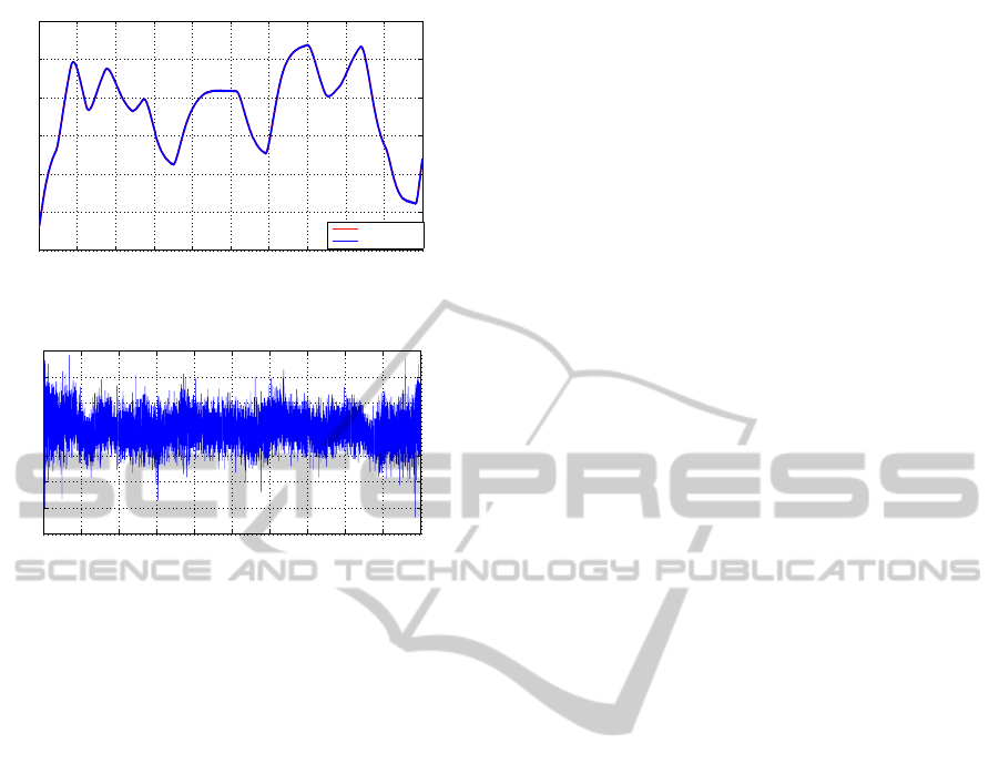
training. The Figure 5, shows the excitation signal
and system response, used in the global training.
0 500 1000 1500 2000 2500 3000 3500 4000 4500 5000
0
5
10
15
20
25
3030
Samples
Level ( Cm )
Response System
0 500 1000 1500 2000 2500 3000 3500 4000 4500 5000
1
1.5
2
2.5
3
3.5
Samples
Voltage ( V )
Excitation signal
Figure 5: Collection of data.
The global model contains four bell-shaped mem-
bership functions, the initialization of membership
functions was the grid partion, for the case that
only has an auxiliary variable, this variable goes
through all the membership functions, as in the case
of two auxiliary variables, each variable involves two
membership functions. The training algorithm used
was backpropagation with the inicial learning rate in
0.001, since the rate is adaptive. The stopping crite-
rion chosen was 1000 epochs or 1×10
−4
of RMSE.In
table 4 below you can see the validation error of
global model identified.
Table 4: Validation of global models.
Aux. Variable Order RMSE Validation Error
L
2
1 0.0317 0.0296
L
2
2 0.0302 0.0289
U 1 0.0330 0.0317
U 2 0.0326 0.0326
L
2
& U 1 0.0317 0.0297
L
2
& U 2 0.0302 0.0289
As can be seen from table 4, the identified models
have proved satisfactory. The difference between the
RMSEs and the validation error is small even consid-
ering the many types of second order compared to the
first order, ie, the choice of a first-order model is bet-
ter because it simplifies the identification as a whole
and also reduces the computational cost. Simplifying
identification, note that the L
2
auxiliary variable
had the lowest RMSE and validation, showing the
model is more efficient. Then we can see the final
result of tune membership functions, that is, after
training using the backpropagation algorithm. First
is plotted the membership functions, for when the
local model is first order, as well as the parameters
of the membership functions, is plotted after the
second order and the parameters of the membership
ICINCO2015-12thInternationalConferenceonInformaticsinControl,AutomationandRobotics
592
functions.
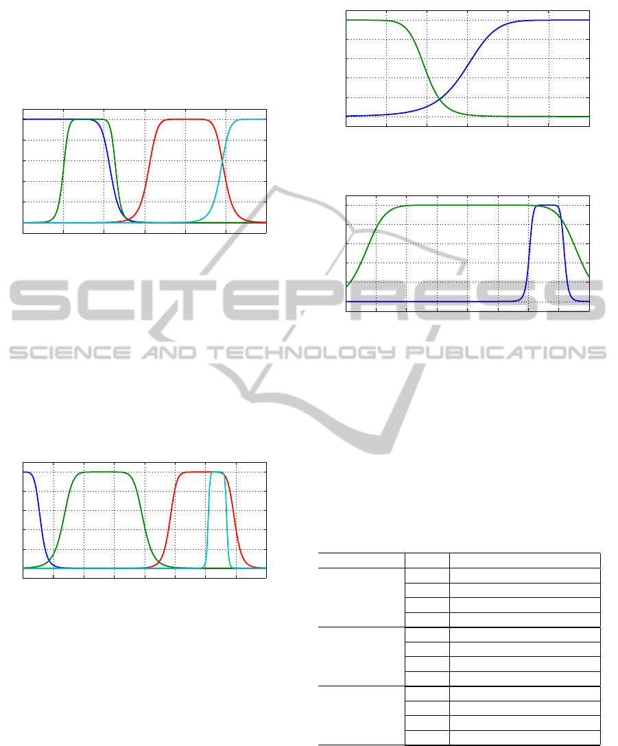
Membership function of modified ANFIS with vari-
able auxiliary L
2
and local models of first order, is
show on figure 6.
0 5 10 15 20 25 30
0
0.2
0.4
0.6
0.8
1
Water Level 2
Degree of membership
C1 C2 C3 C4
Figure 6: Tuned membership functions, first order, variable
auxiliary L
2
.
Analyzing the distribution of the membership
functions of the figure 6 , we can observe that the C
2
membership function is practically in C
1
, implying
that two rules are being used simultaneously in this
range, ie, both are important in this region.
Membership function of modified ANFIS with vari-
able auxiliary U and local models of first order, figure
7.
0 0.5 1 1.5 2 2.5 3 3.5 4
0
0.2
0.4
0.6
0.8
1
Voltage (V)
Degree of membership
C1
C2 C3 C4
Figure 7: Tuned membership functions, first order, variable
auxiliary U.
Observing figure 7, can be noted that the member-
ship function C
4
operates in a small strip and is still
contained in membership function C
3
, implying that
this region is necessary to use two models to achieve
a satisfactory response.
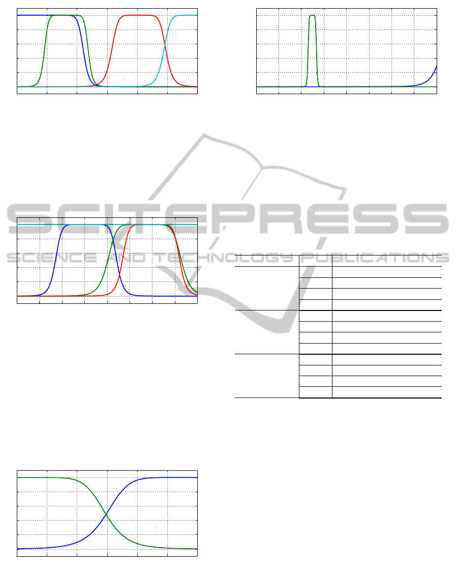
Membership function of the modified ANFIS with
variable auxiliary L
2
&U and local models of first
order,can be seen at figure 8 and 9.
In figure 8 and 9 because the distribution of
the membership functions, that when we are using
two auxiliary variables, the auxiliary variable most
significant has a better distribution. In this case
with the distribution of the membership functions of
0 5 10 15 20 25 30
0
0.2
0.4
0.6
0.8
1
Water Level 2 (cm)
Degree of membership
C2C1
Figure 8: Tuned membership functions L
2
, first order, vari-
able auxiliary L
2
&U.
0 0.5 1 1.5 2 2.5 3 3.5 4
0
0.2
0.4
0.6
0.8
1
Voltage (V)
Degree of membership
D2
D1
Figure 9: Tuned membership functions U, first order, vari-
able auxiliary L
2
&U.
L
2
, noted in range of 5 to 20 cm begin to have the
intersections of the membership functions, implying
that in this range of values are required to use two
models to get a satisfactory response, unlike the
auxiliary variable U, where a small range of values
are necessary to use two models.
In table 5,are show the parameters of the membership
functions for first-order models.
Table 5: Membership Functions first order.
Aux. Variable M.Fs. Coefficient
C
1
[7.1428 6.4285 3.6568]
L
2
C
2
[3.2446 4.8170 8.2258]
C
3
[4.6598 4.0548 20.1214]
C
4
[5.1140 4.4732 29.4848]
C
1
[0.4034 4.0289 -0.1135]
U
C
2
[0.6563 3.9998 1.3212]
C
3
[0.5309 4.5379 2.9468]
C
4
[-0.1526 5.3381 3.1970]
C
1
[12.1111 5.5156 -2.3279]
L
2
& U
C
2
[15.1054 3.9358 29.9124 ]
D
1
[1.7458 5.2769 2.06597]
D
2
[0.2878 4.5000 3.3052]
Membership function of the modified ANFIS with
variable auxiliary L
2
and local models of second or-
der, can be seen at figure 10.
Note figure 10 is very close figure 6 , the C
2
membership function of figure 10 is a little more
open about the membership function of figure 6’s C
2
.
Probably this small opening helped the second-order
NonlinearSystemIdentificationbasedonModifiedANFIS
593
0 5 10 15 20 25 30
0
0.2
0.4
0.6
0.8
1
Water Level 2 (cm)
Degree of membership
C1
C2 C3
C4
Figure 10: Tuned membership functions, second order,
variable auxiliary L
2
.
model has a small improvement over the first order.
Membership function of the modified ANFIS with
variable auxiliary U and local models of second or-
der, figure 11.
0 0.5 1 1.5 2 2.5 3 3.5 4
0
0.2
0.4
0.6
0.8
1
Voltage (V)
Degree of membership
C1 C2
C3
C4
Figure 11: Tuned membership functions, second order,
variable auxiliary U.
Analyzing the distribution of membership func-
tions of the figure 11, we can observe that the
C
4
membership function have degree one for the
entire universe of discourse, ie, this model is always
contributed to get a satisfactory response.
Membership function of the modified ANFIS with
variable auxiliary L
2
& U and local models of second
order, can be seen at figure 12 and 13.
0 5 10 15 20 25 30
0
0.2
0.4
0.6
0.8
1
Water Level 2 (cm)
Degree of membership
C2
C1
Figure 12: Tuned membership functions L
2
, first order, vari-
able auxiliary L
2
&U.
As can be seen in figure 12 and 13, because the
distribution of the membership functions, the L
2
auxiliary variable is practically alone in influencing
0 0.5 1 1.5 2 2.5 3 3.5 4
0
0.2
0.4
0.6
0.8
1
Voltage (V)
Degree of membership
D2D1
Figure 13: Tuned membership functions U, first order, vari-
able auxiliary L
2
&U.
systems, as the auxiliary variable U stay with degree
of membership nearly zero for almost all signals,
giving understand that this variable auxiliary can be
eliminated.
In table 6, We can see the parameters of the mem-
bership functions for second-order models.
Table 6: Membership Functions second order.
Aux. Variable M.Fs. Coefficient
C
1
[6.8437 7.3526 4.216]
L
2
C
2
[3.6495 5.2303 8.2199]
C
3
[4.5231 4.0712 20.2577]
C
4
[5.1006 4.4761 29.5083]
C
1
[0.6797 4.9155 1.5348]
U
C
2
[0.8154 4.0786 2.8290]
C
3
[0.6360 4.4164 2.9728]
C
4
[-36.3879 4.1613 3.3451]
C
1
[14.8221 4.0758 -0.1267]
L
2
& U
C
2
[15.0364 3.9921 29.9672]
D
1
[-0.0931 4.8961 1.2454]
D
2
[0.9008 4.0225 5.0098]
The results obtained with the ANFIS modified’s
auxiliary variable L
2
and first-order models in con-
sequent proved better in a general context, we will
analyze its validation curve and the validation error.
The validate of the modified ANFIS, it was made
a test with the open-loop system where a PRS excita-
tion signal with amplitude varying from 0 to 4 volts
was generated, the modified ANFIS was feedback to
the output of the plant. In the figure 14 shows a graph-
ical comparison of real solution (blue line), modified
ANFIS’s output (red line).
As can be seen in figure 14, the modified ANFIS
able to identify the dynamics of the plant with an er-
ror considered small for the dimensions of the tanks
coupled system. For a more detailed analysis, we can
observe in the figure 15, which helps us to realize the
error in every moment.
By analyzing figure 15, we see that the highest
value of instantaneous error was approximately -0.15
ICINCO2015-12thInternationalConferenceonInformaticsinControl,AutomationandRobotics
594
0 1000 2000 3000 4000 5000 6000 7000 8000 9000 10000
0
5
10
15
20
25
30
Time (s)
Level ( cm )
ANFIS Modified
Real
Figure 14: Validation of the modified ANFIS.
0 1000 2000 3000 4000 5000 6000 7000 8000 9000 10000
−0.2
−0.15
−0.1
−0.05
0
0.05
0.1
0.15
Samples
Error
Figure 15: The modified ANFIS validation error.
cm. Regarding the dimensions of the tank a -0.15 cm
error is a percentage error of 0.5% which is accept-
able depending on the specications. Other error val-
ues vary in the range of approximately -0.2 to 0.2 cm
which represents a percentage of 1%.
4 CONCLUSIONS
The identification of the models, shown in the result
session, using the modified ANFIS shows the impor-
tance of choosing the auxiliary variable. The appro-
priate choice of the variable auxiliary consistent with
the problem can simplify the identification, removing
other variables that have little or no influence on the
system. It was also shown the importance of order of
the model consequent. As seen in the results are not
always increased in the order of local models imply
significant improvements systems.
Due the flexibility and simplicity of modified AN-
FIS method was observed several advantages over
ANFIS, since the dissociation of the inputs to the first
and fifth layer, the method makes it possible to con-
duct training of models which would be unfeasible
with ANFIS due the large computational effort. With
the dissociation of first and fifth layer is also possible
to increase the accuracy of model without increasing
the number of rules, that is, a more accurate system
without significantly increasing the computational ef-
fort.
As seen from the results of the modified AN-
FIS identification method achieved satisfactory re-
sults, since it has small error values for training and
validation, showing its potential for use in identifica-
tion of non-linear systems.
ACKNOWLEDGEMENTS
ANP, MCT, FINEP and by Petrobras financial support
through project PFRH-220.
REFERENCES
Apkarian, J. (1999). Coupled Water Tank Experiments
Manual. Canada.
Babuka, R. (2003). Neuro-fuzzy methods for modeling
and identification. In Recent Advances in Intelligent
Paradigms and Applications.
Fonseca, C. A. G. (2012). Estrutura ANFIS Modifi-
cada para Identificao e Controle de Plantas com Am-
pla Faixa de Operao e no Linearidade Acentuada.
Doutorado, UNIVERSIDADE FEDERAL DO RIO
GRANDE DO NORTE - UFRN.
Haykin, S. S. (2001). Redes Neurais. Bookman Companhia
Ed, 2nd edition.
Jang, C.-T. S. E. M. (1997). Neuro-fuzzy and soft comput-
ing A Computation Approach to Learn and Machine
Intelligence. Prentice- Hall.
Jang, J.-S. R. (1993). Anfis: Adaptive-network-based fuzzy
inference system. In IEEE Transactions on Systems,
Man and Cybernetics.
Jang, J. S. R. and Sun, G. T. (1995). Neuro-fuzzy modeling
and control. In IEEE.
ZhixiangHow, QuntaiShen, H. (2003). Nonlinear system
identificationbased on anfis. In International Confer-
ence on Neural Networks & Signal Processing.
NonlinearSystemIdentificationbasedonModifiedANFIS
595
