Analysis of Hump Operation at a Railroad Classiﬁcation Yard

Maria Gisela Bardossy

Information Systems and Decision Science, University of Baltimore, 1420 N. Charles Street, Baltimore, U.S.A.

Keywords:

Simulation, Hump Sequencing, Priority Rules, Classiﬁcation Yard, Discrete-event Simulation.

Abstract:

Railroad classiﬁcation yards play a signiﬁcant role in freight transportation: shipments are consolidated to

beneﬁt from economies of scales. However, the disassembling of inbound trains, the classiﬁcation of railcars

and reassembling of outbound trains add signiﬁcant time to the overall transportation. Determining the op-

erational schedule of a railroad classiﬁcation yard to ensure that railcars pass as quickly as possible through

the yard to continue with their journey to their ﬁnal destination is a challenging problem. In this paper, we

create a simulation model to mimic the dynamics of a classiﬁcation yard and investigate the effect of two

simple but practical priority rules (train length and arrival time) for the sequencing of inbound trains through

the humping operation. We monitor the effect of these rules on performance measures such as average wait

time (dwell time) at the yard and daily throughput as the complexity and frequency of the trains vary. We run

the simulation on four data sets with low and high complexity of trains and low and high frequency of trains.

1 INTRODUCTION

Classiﬁcation yards take the role of hub in railroad

networks. Shipments are consolidated to beneﬁt from

economies of scales and full journeys are fragmented

in shorter journeys, which might include one or more

classiﬁcation yards. Classiﬁcation yards add time to

the total length of the journey, in many cases idle

time. Bontekoning and Priemus (2004) state that in

Europe, classiﬁcation yard operations may take 10-

50% of trains total transit time.Dirnberger and Barkan

(2007) pointed classiﬁcation yard as an area of high

potential for total transit time improvement. However,

there are a number of working components in the op-

eration of a classiﬁcation yard that can lead to chal-

lenges in its potential optimization. In particular, the

humping sequence as it is most crucial and directly

inﬂuences the outbound trains departure times, Jaehn

et al. (2015). Eggermont et al. (2009) noted the hard-

ness of train rearrangement even in the most simple

layouts. There are two types of classiﬁcation yards:

ﬂat and hump. On hump yards there is track on a

small hill over which a hump engine pushes the cars,

which are then directed using switches to the appro-

priate classiﬁcation track. Our study concentrates on

hump classiﬁcation yards. Armstrong (1990) provide

a throughout description of railroad operations.

For the purpose of analysis, following we provide

a concise description of a hump classiﬁcation yard

and its most salient operational characteristics. Most

Figure 1: Layout of a typical classiﬁcation yard.

classiﬁcation yards have three major sections, shown

in Figure 1, that make up its structure: the receiving

area, the classiﬁcation area, and the departure area.

Each region of the yard plays a role in moving the

cars to its respective terminal. Once an inbound train

is received, the train is directed to an available receiv-

ing track for inspection. During this time, the loco-

motive is removed from the train and the railcars are

processed in the receiving area.

After inspection is complete, the cars are approved

for transfer into the classiﬁcation area. In order to

reach the classiﬁcation tracks, an engine is used to

propel the railcars from the selected receiving track

over the hump towards the classiﬁcation area. Cars

that are enroute to the same destination are grouped

together to create a block. A number of switches are

used to move blocks from the hump to the appropriate

classiﬁcation track. An ideal situation would be for

each block to have its own classiﬁcation track. How-

ever, due to capacity limitations of the yard, multiple

blocks may be required to use the same classiﬁcation

track.

The classiﬁcation area stores the inventory of

493

Bardossy M..

Analysis of Hump Operation at a Railroad Classiﬁcation Yard.

DOI: 10.5220/0005546704930500

In Proceedings of the 5th International Conference on Simulation and Modeling Methodologies, Technologies and Applications (SIMULTECH-2015),

pages 493-500

ISBN: 978-989-758-120-5

 2015 SCITEPRESS (Science and Technology Publications, Lda.)

rail cars available for assembly into outbound trains.

Once the predetermined amount of railcars needed for

an outbound train become available, an engine will

move into the classiﬁcation area. The engine will then

take the necessary blocks from one or more tracks

and arrange them in a distinct order. After the cars

are lined up in the appropriate order, the newly as-

sembled outbound train is pulled into an available de-

parture track. It is at this point that the locomotive is

reattached and a ﬁnal inspection of the railcars is com-

pleted before the outbound train leaves the departure

area.

Railroad yard operations are focused on making

connections between inbound trains and outbound

trains. The yardmaster is responsible for generating

a plan that manages these movements while ensuring

that all operational constraints are met. Our goal is

to characterize the effect of simple but practical pri-

ority rules such as FIFO (ﬁrst in ﬁrst out) and total

hump time on yard performance measures such as av-

erage wait time and daily throughput as the complex-

ity and frequency of the train vary. The sequence in

which trains are hump has a downstream effect on the

outbound trains. That effect can be soothed or am-

pliﬁed by characteristics of the ﬂow of inbound trains

as well as operational constraints of the yard such as

the number of classiﬁcation tracks. The rest of this

paper is organized as follows. In 2 we review prior

optimization work on railroad operations and on se-

quencing at the hump in particular. In 3 we survey the

classiﬁcation yard operations and present a discrete-

event simulation model. In 4 we describe four data

sets of inbound trains with distinct characteristics in

terms of the complexity of the inbound trains and in-

terarrival rate. In 5 we characterize the effect of the

priority rules on yard performance measures such as

average wait time (or dwell time) and daily through-

put. In addition, we discuss how these insights can

modeled operational decisions in train sequencing. 6

provides concluding remarks and directions for future

research.

2 LITERATURE REVIEW

Optimization of railroad operations has received re-

vived attention in the last years. The Railway Ap-

plication Section (RAS) from the Institute for Op-

erations Research/Management Science (INFORMS)

has contributed to direct operation research (OR)

academics and practitioners’ attention to challeng-

ing problems in the ﬁeld (INFORMS, 2015). Since

2010 each year RAS has partnered with leaders in the

ﬁeld to sponsor research competitions on challenging

questions in railroad operations. Railroad yard oper-

ation in particular was their 2013 challenge problem.

Earlier works on this problem had mostly focused on

high-level analytical models; these initiatives in con-

trast seek to drill down to the speciﬁcs and provide

detailed solutions to these operational decisions.

Boysen et al. (2012) provides a thorough review of

the literature in the last 40 years. The focus is on sort-

ing strategies and identifying research opportunities

in the ﬁeld. The work presented in this paper closely

relates to Kraft (2002), He et al. (2003), Hansmann

and Zimmermann (2008), M

arton et al. (2009), and

Jaehn et al. (2015) as it concentrates in the detailed

scheduling decisions for disassembling and reassem-

bling of trains. He et al. (2003) propose a mixed 0-

1 programming formulation and a decomposition op-

timization solution method to determine the optimal

decisions. They consider a model with a single hump

engine and with set outbound train schedules. Their

model objective is to minimize train delays and depar-

tures from the outbound train schedule. While M

arton

et al. (2009) combine an integer programming ap-

proach and a computer simulation tool to successfully

develop and verify an improved classiﬁcation sched-

ule for a real-world train classiﬁcation instance. They

derive the scheduling program from a bitstring repre-

sentation which it includes all the restrictions from a

Swiss classiﬁcation yard. Jaehn et al. (2015) inves-

tigates also the optimal humping sequence in order

to minimize a weighted tardiness of outbound trains.

They show that the problem is NP-hard and present a

mix integer programming formulation.

Describing earlier work, Cordeau et al. (1998)

presents a survey of optimization models for the most

commonly studied rail transportation problems. A

whole section is dedicated to analytical yards models

highlighting the importance of the problem in railroad

operation. In the majority of the papers reviewed by

the authors, the model of choice is a queuing model

and the main objective is to understand the impact

of different strategies on the transit times at a policy

level.

Keaton (1989) explains that car time in interme-

diate terminals occurs in classiﬁcation and assembly

operations and while waiting for the departure of an

outbound train, but also as a result of yard congestion.

Earlier, Crane et al. (1955) presents an analysis of a

particular hump yard and discussed the queuing pro-

cesses identiﬁed in inspection and classiﬁcation oper-

ations. A model for the location of a classiﬁcation

yard was proposed by Mansﬁeld and Wein (1958).

Petersen (1977a,b) develops queuing models to rep-

resent the classiﬁcation of incoming trafﬁc and the

assembly of outbound trains. In these queuing mod-

SIMULTECH2015-5thInternationalConferenceonSimulationandModelingMethodologies,Technologiesand

Applications

494

els, the author observed that the delay between end

of classiﬁcation to start of assembly is a minor source

of yard congestion in comparison with classiﬁcation

and assembly operations. A thorough description of

railyards is presented in the ﬁrst paper.

Turnquist and Daskin (1982) models yard opera-

tions from the perspective of freight cars and devel-

oped queuing models for classiﬁcation and connec-

tion delays that consider individual cars as the basic

units of arrival. Martland (1982) described a method-

ology for estimating the total connection time of cars

passing through a classiﬁcation yard. The model is

based on a function, ﬁtted using actual data from the

railroad, that relates the probability of making a par-

ticular train connection to the time available to make

that connection and other variables such as trafﬁc pri-

ority and volume.

In terms of sorting strategies and block-to-

classiﬁcation track assignment, Siddiqee (1971) com-

pares four sorting and train formation schemes in a

railroad hump yard. Yagar et al. (1983) proposes

a screening technique and a dynamic programming

approach to optimize humping and assembly opera-

tions. They propose an algorithm consisting of two

main components: a screening technique and a de-

tailed cost minimization procedure for the humping

and assembly phases. Daganzo et al. (1983) inves-

tigated the relative performance of different multi-

stage sorting strategies. In multistage sorting, several

blocks are assigned to each classiﬁcation track, and

cars must be resorted during train formation. More

recently, in multistage sorting Jacob et al. (2011) de-

velops a novel encoding of classiﬁcation schedules,

which allows characterizing train classiﬁcation meth-

ods simply as classes of schedules. Avramovi

c (1995)

models the physical process of cars moving down the

hump of a yard. This process is represented by a sys-

tem of differential equations that incorporate several

factors, such as hump proﬁle and rolling resistance,

affecting the movement of a car.

The simulation model presented here draws from

some of the ﬁndings presented in these earlier papers.

Yagar et al. (1983) also considers a FIFO strategy for

the humping; however, it does not investigate how the

performance of each strategy is correlated to the ﬂow

of the inbound trains. The purpose of the analysis

here goes beyond proposing priority rules to under-

stand the dynamics of the ﬂow of trains jointly with

the priority rules. In order to concentrate our atten-

tion, we have decided to relegate for now aspects such

as sorting decisions (Daganzo et al., 1983) and distri-

bution of times (Martland, 1982).

3 HUMP OPERATION AND

SIMULATION MODEL

The operations of a classiﬁcation yards is modeled us-

ing a discrete-event simulation model. Given a ﬂow

of inbound trains, the model determines when incom-

ing trains are humped and moved through the yard to

outbound trains. There is no outbound train schedule

pre-deﬁned, the outbound train schedule is deﬁned by

the model and the decisions made in the process.

The model is based on the following assumptions:

• The classiﬁcation sequence of the inbound trains.

When the number of inspected trains in the re-

ceiving yard exceeds one, the model determines

which train should be humped next. This is es-

pecially important to ensure that incoming trains

ﬁnd an open receiving track while grouping the

necessary blocks for the outbound trains. Shortest

trains require less time to hump which frees up re-

ceiving tracks quicker but limits the construction

of outbound trains.

• The assembly sequence of the outbound trains.

When the number of cars to form a unit or com-

bination train in the classiﬁcation area exceeds a

certain number (minimum number of cars deter-

mined by the operational constraints), the pull-

back engine can assemble the string of cars into

an outbound train. When there are multiple po-

tential outbound trains, the model has to deter-

mine which train to pullback. In the given speci-

ﬁcations there are two identical pullback engines,

so while the model determines which engine pulls

the train it is not critical for the operational plan.

In our model, there are additional operating char-

acteristics that were established beforehand:

• Scheduling is non preemptive. Once a humping

job is started it cannot be interrupted until all the

railcars in the train have been completely humped.

Similarly, the assembling of outbound trains can-

not be interrupted; all tracks that will form the out-

bound train must be pulled sequentially and with-

out delay between pullbacks.

• Block-to-track assignment is dynamic. Blocks are

assigned to tracks as they are necessary. Empty

tracks become available immediately to whatever

block requires them.

• Block-to-track assignment follows a decreasing

order. When multiple classiﬁcation tracks store

the same block type, new cars are ﬁrst assigned

to the track with the highest inventory up to reach

capacity. Similarly, when a track of a block type

needs to be pulled, the track with the most railcars

is pulled ﬁrst.

AnalysisofHumpOperationataRailroadClassificationYard

495

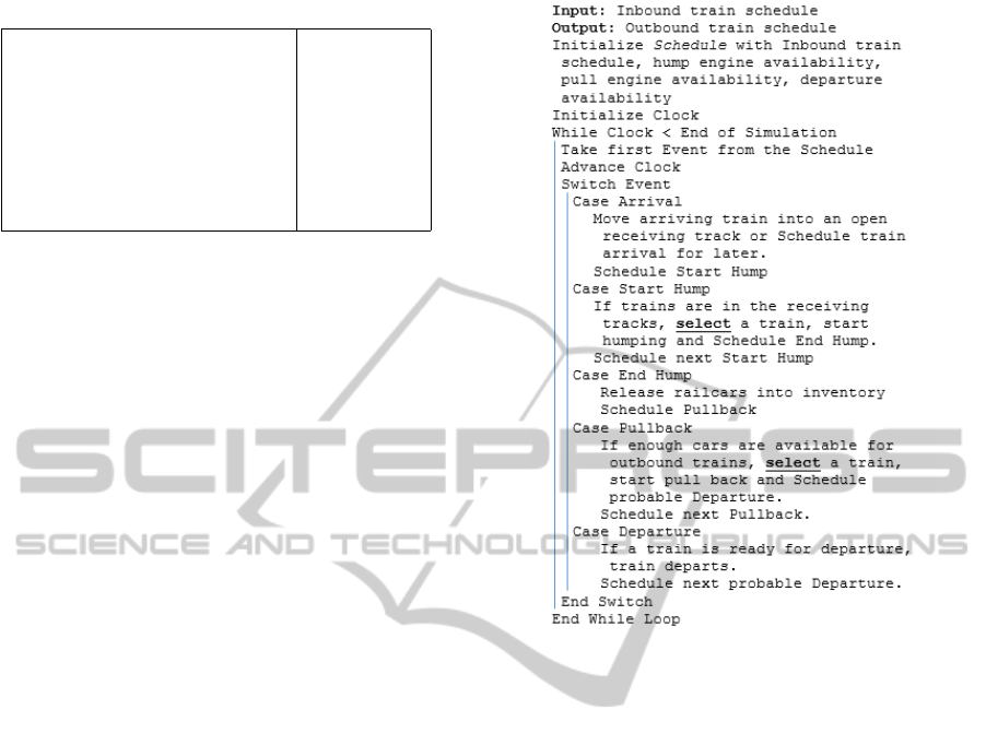
Table 1: Operational Constraints.

Receiving tracks (capacity) 10 (185)

Classiﬁcation tracks (capacity) 42 (60)

Departure tracks (capacity) 7 (207)

Inspection time 45 min

Hump rate 2.2 cars/min

Interval between humping jobs 10 min

Hump engines 1

Pullback engines 2

• Hump and pullback engines cannot be idle while

trains wait. While theoretically engines could

await for better trains to hump or pull back, in our

model that is not allowed. If the hump engine be-

comes available and there are trains waiting in the

receiving area, the engine must immediately start

humping the next train. Similarly, if a pullback

engine becomes available and there are enough

railcars to form an outbound train, the engine will

commence to pullback the available unit or block

combination.

Other operating constraints such as the number

of receiving, classiﬁcation, and departure tracks, in-

spection time, and interval between humping jobs are

shown in Table 1. In the next section, we brieﬂy de-

scribe some characteristics of the inbound trains in

each dataset. Figure 2 highlights the core of the simu-

lation model where a Schedule list keeps track of each

of the events that take place and a Clock subsequently

advances as the simulation progresses.

There are train arrivals, humping, pulling and de-

partures that interact through state variables such as

the state of tracks, engine and location of railcars. In

this simulation model, there is one spot time when a

decision -select a train- with consequences that will

cascade through the system take place. For those de-

cisive moments, we identify some decision rules. We

develop rules for prioritizing the humping of trains in

the receiving area and the construction of outbound

trains. These guidelines determine the order that in-

bound trains should be humped when more than one

train is present in the receiving area, the classiﬁca-

tion tracks required to pull the selected block combi-

nation, and secures the necessary inventory for out-

bound train departure.

Humping Rules:

We concentrate in two simple but practical crite-

ria: the idle time in the receiving area and the hump-

ing time required by the train. The idle time in the

receiving area represents the amount of time that the

train has been ready (after inspection) and waiting for

humping while the humping time is a function of the

train length. The idle time can be used as a ﬁrst in ﬁrst

out (FIFO) criterion. This queue discipline is often re-

Figure 2: Simulation Pseudocode.

ferred as the fairest as it achieves the lowest variance

in waiting times. On the other hand the hump time

can be used for a shortest train ﬁrst criterion or longest

ﬁrst criterion. The rationale for Shortest Train First is

that an inbound train in the receiving area, regardless

of the length, occupies the entire receiving track, and

under certain circumstances humping shorter trains

ﬁrst to quickly free up a track for incoming trains

might yield a decreased chance of rescheduling in-

bound trains and improving performance measures.

A disadvantage to humping the shortest train is its

eventual limitations to generate outbound trains due

to a lack of acceptable block combinations. Similarly,

the rationale for Longest Train First is longer trains

increase the number of potential outbound train com-

binations that will be available in the next stage of the

rail yard.

At the time of humping all ready to hump trains

are given a score, s, that depends on the amount of

time that the trains has been in the receiving area, w,

and the amount of time that it would take to complete

the hump job for the train, l. Both times are mea-

sured in minutes. The total score is the sum of both

time multiplied respectively by an importance weight.

Then, the train with the highest score is humped (dis-

carding any train that would not ﬁt in the classiﬁcation

tracks.)

SIMULTECH2015-5thInternationalConferenceonSimulationandModelingMethodologies,Technologiesand

Applications

496

Table 2: Summary Train Information.

Feature Dataset 2 Dataset 3 Dataset 4 Dataset 5

Blocks 13 13 33 33

Inbound Trains 339 491 339 491

Trains per Day 19 27 19 27

Train Length 70 72 70 72

Total Railcars 24330 34130 24330 34130

Cars per Day 1352 1896 1352 1896

Interarrival Time 1:16 0:52 1:16 0:52

Hump Cycle 0:42 0:43 0:42 0:43

Common Block AH AH AH AH

Rare Block BG BG AO AO

s = α ∗ w + β ∗ l (1)

where α and β are the respective weights.

Pullback Rules:

For pullback operations, we select the longest pos-

sible outbound train regardless the amount of time

that it requires to assemble. This might be suboptimal

since unit trains are faster to assemble and pull than

combination trains and the gain in a longer train might

be lost when the time factor is considered. Anyway,

we choose this strategy since its simplicity allows to

observe more clearly the effect of humping rules.

4 DESCRIPTION OF INBOUND

TRAINS

Five distinct data sets of inbound trains where ana-

lyzed. Data set 1 was used to test the functionality of

the simulation model. Data sets 2 and 3 have a lim-

ited number of incoming blocks (13 blocks) and block

combinations (5 combinations), fewer trains per day

and fewer railcars per day; whereas data sets 4 and 5

are more comprehensive with 33 blocks, more com-

binations (13 combinations) and more daily trains.

While the data sets had their own randomly gen-

erated inbound train combinations, there were sev-

eral similarities between them. On average, the train

length for each data set was approximately the same

at 70 cars per train. In addition, the interarrival times

of the trains were relatively consistent in its sequence.

Each data set consists of 18 days of inbound trains.

As shown in Table 2, the data sets presented sim-

ilar patterns within its measurements. The major dif-

ferences between the data sets comes from the in-

creased variety of blocks applicable to the full data

sets. The modiﬁcation in the assortment of blocks

spread across the same amount of railcars in each data

set causes a smaller volume of each block to be avail-

able for outbound trains. There are not notable dif-

ferences between incoming trains in terms of their

constitution. Most trains have at least one railcar of

each block type; consequently, more blocks translate

to diversiﬁed trains with few blocks of each type and

Table 3: Summary Results 1.

Data set 2 Data set 3

Measure min max min max

Dwell Time 1.137 1.200 0.889 0.965

Delayed Trains 0 0 8 16

Daily Throughput 1344.69 1345.85 1818.71 1845.16

Hump Utilization 55% 56% 76% 77%

Pullback Utilization 47% 51% 65% 69%

Table 4: Summary Results 2.

Data set 4 Data set 5

Measure min max min max

Dwell Time 2.688 2.785 2.434 2.541

Delayed Trains 0 0 8 16

Daily Throughput 1343.24 1346.07 1820.15 1848.93

Hump Utilization 55% 56% 76% 77%

Pullback Utilization 71% 75% 87% 89%

longer times to consolidate the minimum number of

railcar to assemble an outbound train. In other words,

based on this information we expect the cycle time to

assemble trains in data set 3 and 5 to be considerably

longer than in data set 2 and 4. Our model will assist

to deﬁne whether more emphasis should be given to

wait time or the length of the train in either case.

5 COMPUTATIONAL

EXPERIMENT AND

CHARACTERIZATION OF

RESULTS

We are going to report on a set of performance mea-

sures to compare the different priority rules. We vary

the weight for wait time and hump time between -

2 to 2 in steps of 0.2. A negative weight indicates

that such dimension is given an inverse importance;

for example, instead of longest train ﬁrst, the shortest

train goes ﬁrst. The performance measures consid-

ered are the following:

Arrivals: On time arrivals of inbound trains are

essential in order to ensure that a continuous ﬂow of

railcars is available for departure. The rescheduling of

an inbound train for a later time prevents the contents

of that train from being available as expected which

ultimately affects other events occurring within the

system. Delays evaluate how closely the simulation

meets the given inbound train schedule. At the end of

the simulation, the model compares the time stamps

of the inbound trains to their expected arrival times.

It then calculates the total number of trains that were

processed and if the output matches the pre-scheduled

times. This information is useful in determining how

often the receiving area is occupied versus available.

Hump Engine: The hump engine plays a vital role

AnalysisofHumpOperationataRailroadClassificationYard

497

-2 -1.5 -1 -0.5 0 0.5 1 1.5 2

-2

-1.5

-1

-0.5

0.5

1.5

Weight for Wait Time

Average Dwell Time for Dataset 2

Weight for Hump Time

Figure 3: Dwell time Data set 2.

in limiting arrival time delays by ensuring the receiv-

ing tracks are available for future incoming trains.

To accomplish this task, the hump engine should be

working to eliminate the pending workload in the re-

ceiving area. By studying the waiting times of in-

bound trains housed in the available receiving tracks,

we are about to evaluate how effectively the hump en-

gine is working. Our objective is to maximize the uti-

lization rate of the hump engine while minimizing the

time a railcar must occupy the receiving area.

Classiﬁcation Tracks: Proportion of classiﬁcation

tracks that are used at its peak; that is, the maximum

proportion of the current tracks that are ever used.

Overall average proportion of time that classiﬁcation

tracks are in use; that is time that used tracks are used

divided by the total available time. This is only for

the percentage of tracks that are ever occupied.

Pullback Engines: Expediting the removal of rail-

cars from the classiﬁcation area adds more space for

incoming rail cars. The examination of the actions of

the pullback engine monitors the process of eliminat-

ing rail cars within the system. In reviewing how the

pullback engines are managed, we should have more

data to evaluate the strength of corresponding strat-

egy.

Departure: Once an outbound train has been

pulled into the departure area, statistical data is gen-

erated in reference to its contents. Details such as the

number of railcars, the block combination, and classi-

ﬁcation tracks pulled are used to gauge the character-

istics of the outbound trains.

Dwell Time: Dwell time is time difference be-

tween when a rail car enters the classiﬁcation track

until it departs to the departure area. Satisfying our

objective requires reducing the amount of time a rail

car spends within the classiﬁcation yard. When re-

viewing each simulation, the average dwell time is

utilized to measure the potential beneﬁts of the strat-

egy in question. We started with a base case deﬁned

as FIFO priority for humping and longest train ﬁrst

-2 -1.5 -1 -0.5 0 0.5 1 1.5 2

-2

-1.5

-1

-0.5

0.5

1.5

Weight for Wait Time

Average Dwell Time for Dataset 3

Weight for Hump Time

Figure 4: Dwell time Data set 3.

for pullback jobs, which yield considerably good re-

sults for the four data sets in terms of average dwell

time. In the data sets analyzed, the classiﬁcation area

has ample capacity; consequently, the main link be-

tween the humping engine and the pullback engine

is through the ﬂow of railcars that the hump engine

produces in a purely downward direction. The de-

cisions at pullback engine are not transmitted to the

hump engine in an upward direction; the hump engine

is safeguarded of the actions of the pullback engine

thanks to the extra capacity available in the classiﬁca-

tion area.

Tables 3 and 4 summarize the results for the four

data sets. When FIFO in used for humping, for Data

Set 2 and 4 there are no delay arrivals and the ar-

rival, hump engine and classiﬁcation track perfor-

mance measures are identical independently of the

priority rule implemented by the pullback engines. In

Data Set 3 and 5, about 17% of the arriving trains are

delayed depending on the weights given to wait time

and hump time, but again the performance measures

for the arrival and classiﬁcation areas are the same

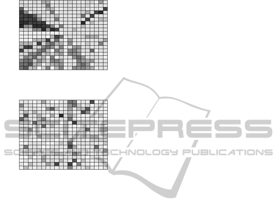
across the different pullback criteria. Figure 3-6 show

how dwell time varies for the different weight values.

The dark areas indicate the most salient performance

either with lowest average dwell time or highest aver-

age dwell times. In Figure 3 and 4 we can observe

some tendency and localize areas. In Figure 3 the

lowest dwell time are concentrated in the vertical cen-

tered area while the highest dwell times are in the

upper left corner. In other words, best dwell times

are observed toward relative positive weight for wait

time and negative weight for hump time. Negative

weight for the hump time indicates that shortest trains

are given priority over longer trains. In Figure 4, the

lowest dwell times are also observed in the center area

but only on the lower part. On the lower left corner

and center upper are dwell times are at their highest.

Figure 5 also shows some distinctive areas. Here

there is no central dominating area. The lowest dwell

SIMULTECH2015-5thInternationalConferenceonSimulationandModelingMethodologies,Technologiesand

Applications

498

-2 -1.5 -1 -0.5 0 0.5 1 1.5 2

-2

-1.5

-1

-0.5

0.5

1.5

Weight for Wait Time

Average Dwell Time for Dataset 4

Weight for Hump Time

Figure 5: Dwell time Data set 4.

-2 -1.5 -1 -0.5 0 0.5 1 1.5 2

-2

-1.5

-1

-0.5

0.5

1.5

Weight for Wait Time

Average Dwell Time for Dataset 5

Weight for Hump Time

Figure 6: Dwell time Data set 5.

times are in the upper area (higher weight for hump

time) and highest dwell time in the bottom area. Fig-

ure 6 does not show such distinctive pattern which

indicates that as the complexity of the inbound trains

increases simple priority rules such as FIFO and train

length (or hump time) become more unpredictable.

Interestingly, we observe that complexity as the num-

ber of blocks has a more signiﬁcant impact than the

frequency of trains. From data set 2 to 3 as the ﬂow

of train increases but with similar complexity the pat-

tern intensiﬁes. In Figure 6 some lowest dwell times

are observed in the upper center area while highest

dwell times are observed in the center lower area. On

the other hand, the priority rule used at the hump en-

gine determines the ﬂow of railcars and practically

deﬁnes the outbound trains and the overall efﬁciency

of the system. There are wide differences in the per-

formance measures across priority rules. The shortest

train ﬁrst yields consistently poor dwell time and high

delays. However, the longest train ﬁrst depending on

the data set yields ranging results: for Data Set 2 it

yields competitive average dwell time and through-

put performance and for Data Set 4 yields the highest

throughput. A disadvantage of Longest First is the

variability in dwell time.

6 CONCLUSIONS

We characterize the performance of two simple pri-

ority rules -FIFO and length of the train- and their

combination through a weighting function that com-

bines them into one simple score to deﬁne the hump-

ing sequence. We observe that neither purely FIFO

nor train length yield the shortest dwell times. In-

stead, a combination of both yields the best perfor-

mance. The weights to obtain the optimal score de-

pends on the characteristics of the ﬂow of incoming

trains. When the number of blocks is low, the optimal

score gives relative importance to the wait time and

negative importance to the length of the train meaning

that shorter trains are given priority. These observa-

tions become even stronger when the ﬂow of trains

increases; that is, when the arrival rate of train in-

creases. On the other hand, the optimal score gives

priority to the length of the train and even a nega-

tive weight to the wait time in the receiving area when

there is a larger number of blocks and a regular ﬂow

of trains. Lastly, the performance for data set 5 is

very sensitive to the weights without a clear pattern

toward the wait time nor the length of the trains. This

further shows the importance of devising optimized

priority rules for humping when the ﬂow is high and

there is great variability of trains. In data set 5, we

observe that small changes in the weights can change

radically whether the best or the worst dwell times

can be attained. A model like the one described here

can assist in the process of discovering and adjusting

the weights as the ﬂow changes. The model present

here can be enhanced to analyze other yards charac-

teristics. For example, it can assist to understand how

the number of classiﬁcation tracks and their capacity

paces the ﬂow of cars through the yard and the re-

lationship between the hump and pullback jobs. In

these data sets the main objective was to minimize

the average dwell time while maximizing through-

put; consequently, the highest achieving rules humped

trains immediately and pull back trains without de-

lay. The utilization rate of engines does not constitute

a bottleneck in these problems and the engines can

be freely assigned. Departure tracks are rarely full

and trains spend minimum time in them. It would

be interesting to analyze the upward effect of a con-

straining number of departure tracks. Our simulation

model provides a ﬂexible framework to test and an-

alyze alternative priority rules for the operation of a

rail yard and yields valuable insight regarding the in-

tricate forces at play.

AnalysisofHumpOperationataRailroadClassificationYard

499

REFERENCES

Armstrong, J. H. (1990). The Railroad: What it is, What it

Does. The Introduction to Railroading.

Avramovi

c, Z.

Z. (1995). Method for evaluating the strength

of retarding steps on a marshalling yard hump. Euro-

pean journal of operational research, 85(3):504–514.

Bontekoning, Y. and Priemus, H. (2004). Breakthrough in-

novations in intermodal freight transport. Transporta-

tion Planning and Technology, 27(5):335–345.

Boysen, N., Fliedner, M., Jaehn, F., and Pesch, E. (2012).

Shunting yard operations: Theoretical aspects and

applications. European Journal of Operational Re-

search, 220(1):1–14.

Cordeau, J.-F., Toth, P., and Vigo, D. (1998). A survey of

optimization models for train routing and scheduling.

Transportation science, 32(4):380–404.

Crane, R. R., Brown, F. B., and Blanchard, R. O. (1955).

An analysis of a railroad classiﬁcation yard. Jour-

nal of the Operations Research Society of America,

3(3):262–271.

Daganzo, C. F., Dowling, R. G., and Hall, R. W. (1983).

Railroad classiﬁcation yard throughput: The case

of multistage triangular sorting. Transportation Re-

search Part A: General, 17(2):95–106.

Dirnberger, J. R. and Barkan, C. P. (2007). Lean railroading

for improving railroad classiﬁcation terminal perfor-

mance: bottleneck management methods. Transporta-

tion Research Record: Journal of the Transportation

Research Board, 1995(1):52–61.

Eggermont, C., Hurkens, C. A., Modelski, M., and Woeg-

inger, G. J. (2009). The hardness of train rearrange-

ments. Operations Research Letters, 37(2):80–82.

Hansmann, R. S. and Zimmermann, U. T. (2008). Optimal

sorting of rolling stock at hump yards. Springer.

He, S., Song, R., and Chaudhry, S. S. (2003). An integrated

dispatching model for rail yards operations. Comput-

ers & operations research, 30(7):939–966.

INFORMS (2015). Railway Applications Section (RAS)

problem solving competition.

Jacob, R., M

arton, P., Maue, J., and Nunkesser, M. (2011).

Multistage methods for freight train classiﬁcation.

Networks, 57(1):87–105.

Jaehn, F., Rieder, J., and Wiehl, A. (2015). Minimizing

delays in a shunting yard. OR Spectrum, 37(2):407–

429.

Keaton, M. H. (1989). Designing optimal railroad oper-

ating plans: Lagrangian relaxation and heuristic ap-

proaches. Transportation Research Part B: Method-

ological, 23(6):415–431.

Kraft, E. R. (2002). Priority-based classiﬁcation for improv-

ing connection reliability in railroad yards. In Journal

of the Transportation Research Forum, volume 56.

Mansﬁeld, E. and Wein, H. H. (1958). A model for the

location of a railroad classiﬁcation yard. Management

Science, 4(3):292–313.

Martland, C. D. (1982). Pmake analysis: Predict-

ing rail yard time distributions using probabilistic

train connection standards. Transportation Science,

16(4):476–506.

arton, P., Maue, J., and Nunkesser, M. (2009). An

improved train classiﬁcation procedure for the hump

yard lausanne triage. In ATMOS.

Petersen, E. (1977a). Railyard modeling: Part i. predic-

tion of put-through time. Transportation Science,

11(1):37–49.

Petersen, E. (1977b). Railyard modeling: Part ii. the ef-

fect of yard facilities on congestion. Transportation

Science, 11(1):50–59.

Siddiqee, M. W. (1971). Investigation of sorting and train

formation schemes for a railroad hump yard. Techni-

cal report.

Turnquist, M. A. and Daskin, M. S. (1982). Queuing mod-

els of classiﬁcation and connection delay in railyards.

Transportation Science, 16(2):207–230.

Yagar, S., Saccomanno, F., and Shi, Q. (1983). An efﬁcient

sequencing model for humping in a rail yard. Trans-

portation Research Part A: General, 17(4):251–262.

SIMULTECH2015-5thInternationalConferenceonSimulationandModelingMethodologies,Technologiesand

Applications

500