Comparison of Robust Control Techniques for Use in Flight Simulator
Motion Bases
Mauricio Becerra-Vargas
GASI, UNESP-Univ Estadual Paulista, Campus Sorocaba, CEP 8087-180, Sorocaba, SP, Brazil
Keywords:
Inverse Dynamics Control, H-Infinity Theory, Sliding Mode Control, Flight Simulator Motion Base, Stewart
Platform, Parallel Robot.
Abstract:
The purpose of this study is to analyse and compare three control strategies based on the inverse dynamics
control structure for a six degree of freedom flight simulator motion base driven by electromechanical ac-
tuators. All strategies are applied in the outer loop of the inverse dynamic control structure by considering
imperfect compensation of the nonlinearities. Imperfect compensation is intentionally introduced in order to
simplify the implementation of the inverse dynamic control structure. The first strategy is just a proportional
and derivative control, the second is based on Lyapunov stability theory and the third is based on H-Infinity
theory. Acceleration step response and smoothness of the actuators driven torques were used to compare the
performance of the controllers. The results are based on numerical simulations.
1 INTRODUCTION
Inverse dynamics control (Sciavicco and Siciliano,
2005; Spong and Vidyasagar, 2006) is an approach
to nonlinear control design whose central idea is to
construct an inner loop control based on the motion
base dynamic model which, in the ideal case, exactly
linearizes the nonlinear system and an outer loop con-
trol to drive tracking errors to zero. This technique
is based on the assumption of exact cancellation of
nonlinear terms. Therefore, parametric uncertainty,
unmodeled dynamics and external disturbances may
deteriorate the controller performance. In addition, a
high computational burden is paid by computing on-
line the complete dynamic model of the motion-base
(Koekebakker, 2001). Robustness can be regained by
applying robust control techniques in the outer loop
control structure as is shown in (Becerra-Vargas and
Belo, 2010; Becerra-Vargas and Belo, 2011; Becerra-
Vargas and Belo, 2012).
In this context, this work presents the comparison
of three control strategies applied in the outer loop
of the feedback linearized system for robust accelera-
tion tracking in the presence of parametric uncertainty
and unmodeled dynamic, which is intentionally intro-
duced in the process of approximating the dynamic
model in order to simplify the implementation of this
approach.
The first strategy is just a proportional and deriva-
tive control applied in the outer loop while the others
two strategies introduce an additional term to the in-
verse dynamics controller which provides robustness
to the control system. In the first strategy, the control
term is designed just by providing stability, in the sec-
ond, through Lyapunov stability theory and the third
strategy through H-Infinity theory.
About organization of the text, this paper is struc-
tured as follows: in Section 2, the full dynamic model
of motion base is presented and the inverse dynamics
structure and imperfect compensation is discussed. in
Section 3 and 4, the imperfect compensation is stabi-
lize through the Lyapunov and H-Infinity theory, re-
spectively, in Section 5 the dynamic model matrices
that will be use in the controllers are defined,in Sec-
tion 6 the results obtained from simulation are shown
and discussed and conclusions of the present work are
discussed.
2 INVERSE DYNAMIC CONTROL
In this study, a six-degree-of-freedom mechanism
called the Stewart platform (Stewart, 1965) is consid-
ered. The UPS (Universal-Prismatic-Spherical) Stew-
art platform is composed of a moving platform linked
to a fixed base through six extensible legs. Each leg
is composed of a prismatic joint (i.e, an electrome-
chanical actuator), one passive universal joint and
344
Becerra-Vargas M..
Comparison of Robust Control Techniques for Use in Flight Simulator Motion Bases.
DOI: 10.5220/0005546803440348
In Proceedings of the 12th International Conference on Informatics in Control, Automation and Robotics (ICINCO-2015), pages 344-348
ISBN: 978-989-758-123-6
Copyright
c
 2015 SCITEPRESS (Science and Technology Publications, Lda.)

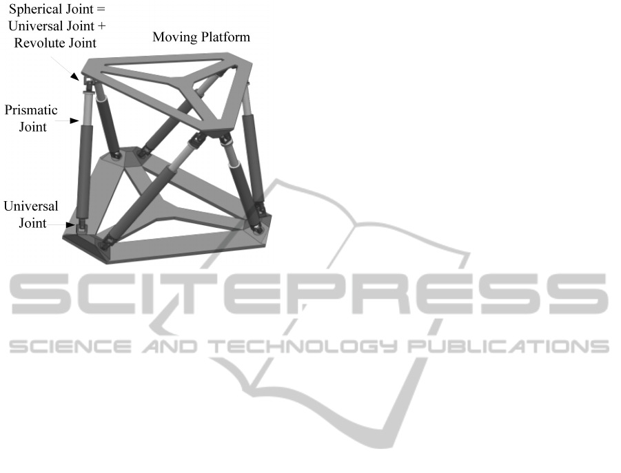
Figure 1: The UPS Stewart Platform.
one passive spherical joint making connection with
the base and the moving platform (Fig. 1), respec-
tively. Usually in flight simulators, due to mechanical
design considerations, such as limited nominal load,
complex design and high friction, spherical joints can
be replaced (kinematically equivalent) by a universal
joint and a revolute joint whose axes intersect and are
non-coplanar as shown in Fig. 1.
The full dynamic model, including the kine-
matic and dynamic of the electromechanical actua-
tor, in Cartesian coordinates can be given as (Becerra-
Vargas and Belo, 2015):
M(q)
¨
q + N(q,
˙
q) = T
m
, (1)
where
N(q,
˙
q) = C(q,
˙
q) + B(
˙
q) + G(q), (2)
and the Cartesian coordinates
q =

x y z φ θ ψ

T
, (3)
and the driving torque generated by the electrome-
chanical actuator
T
m
=

τ
m
1
τ
m
2
τ
m
3
τ
m
4
τ
m
5
τ
m
6

T
(4)
Inverse dynamics control (Sciavicco and Sicil-
iano, 2005; Spong and Vidyasagar, 2006) is a con-
trol law involving two feedback loops: the inner loop,
which, in the ideal case, exactly linearizes the nonlin-
ear system and the outer loop that drives tracking er-
rors to zero. Practical implementation of the inverse
dynamics control requires the parameters of the ma-
trices M(q) and N(q,
˙
q) to be accurately known, the
matrices to be modelled accurately and to be com-
puted in real-time. These requirements are difficult
to satisfy in practice. Model imprecision may come
from parametric uncertainties and purposeful choice
of a simplified representation of the matrices M(q)
and N(q,
˙
q) (unmodeled dynamics intentionally intro-
duced). Therefore, the control law in the imperfect
compensation case can be written as (Becerra-Vargas
and Belo, 2011):
u
T
=
b
M(q)v +
b
N(q,
˙
q); (5)
where u
T
= T
m
represents the vector of voltage
(which is proportional to vector torques, not con-
sidering the actuator electrical dynamics) driving the
servo-drive of the electromechanical actuator, and
b
M,
b
N represent simplified versions of M, N and where
v =
¨
q
d
+ K
d
˙
e + K
p
e,
(6)
and where
K
p
= diag

ω
2
n1
,...,ω
2
n6

;
K
d
= diag
{
2ς
1
ω
n1
,...,2ς
6
ω
n6
}
(7)
and q
d
is the desired Cartesian coordinates and where
the tracking error is defined as
e = q
d
− q, (8)
and ω
ni
and ς
i
characterize the response of the track-
ing error of the inverse dynamics control.
In order to overcome imperfect compensation ef-
fects, in this case, the simplification of the matrices
M and N, a robust term, u, is included in Eq (6), thus
Eq (6) can be written as:
v =
¨
q
d
+ K
d
˙
e + K
p
e + u,
(9)
Now, substituting Eq. (5) into Eq. (1) and simpli-
fying it, one gets (Becerra-Vargas and Belo, 2011):
˙
x = Ax + B(w − u),
(10)
where the state vector x consisting of the error and its
derivative is written as:
x = [
e
˙
e
]
T
,
(11)
and where
w = (I − M
−1
b
M)v − M
−1
∆N
∆N = N −
b
N
(12)
and
A = (H − BK) , K =

K
p
K
d

(13)
and
H =

0 I
0 0

B =

0
I

(14)
ComparisonofRobustControlTechniquesforUseinFlightSimulatorMotionBases
345

3 ROBUST CONTROL TERM, u,
DESIGNED BY LYAPUNOV’S
SECOND METHOD
Robust control term, u, was designed to stabilized the
system represented by the Eq. (10) in the presence of
the uncertainty w, and is given as (Becerra-Vargas and
Belo, 2011)
u =





ρ
k
z
k
z ∀
k
z
k
≥ ε
ρ
ε
z ∀
k
z
k
< ε
(15)
where
z = B
T
Px; (16)
and P is the unique positive definite symmetric solu-
tion of
A
T
P + PA = −T, (17)
and
ρ ≥
1
1 − λ
(λQ
M
+ λ
k
K
kk
x
k
+ B
M
Φ) (18)
sup
t≥0
k
¨
q
d
k
< Q
M
< ∞ ∀
¨
q
d



I − M
−1
b
M



≤ λ ≤ 1 ∀q
k
∆N
k
≤ Φ ≤ ∞ ∀q,
˙
q


M
−1


≤ B
M
∀q
(19)
Although the control law in Eq. (15) does not
guarantee error convergence to zero, it ensures
bounded-norm error given by ε.
4 ROBUST CONTROL TERM, u,
DESIGNED BY H-INFINITY
THEORY
The H-Infinity suboptimal control problem is to find a
stabilizing controller K(s) which, based on the infor-
mation in y, generates a control signal u which coun-
teracts the influence of
e
w on
e
z, thereby minimizing
the closed-loop norm from
e
w to
e
z to less than gamma
via the selected weighting function matrices, that is
(Becerra-Vargas and Belo, 2012)





W
u
(I + KG)
−1
KGW
d
W
e
(I + GK)
−1
GW
d





∞
< γ
(20)
where G(s) is the transfer function of the state space
system defined by Eq. (10), W
e
(s), W
d
(s) and W
u
(s)
represent the weighting functions diagonal matrices
associated with the tracking error, disturbance (uncer-
tainty w in Eq. (12) is considered as disturbance) and
control signal, respectively, and are given as
W
e
=
"
W
e
(s) ··· 0
.
.
.
.
.
.
.
.
.
0 ··· W
e
(s)
#
;W
d
=
"
W
d
(s) ··· 0
.
.
.
.
.
.
.
.
.
0 ··· W
d
(s)
#
W
u
=
"
W
u
(s) ··· 0
.
.
.
.
.
.
.
.
.
0 ··· W
u
(s)
#
(21)
It is observed from Eq. (20) that the transfer
functions, (I + GK)
−1
G and I + KG)
−1
KG, are two-
sided weighted functions, therefore the terms A
s
, A
d
,
A
u
and M
s
, M
d
and M
u
lower and upper bounds the
spectrum of them.
5 CHARACTERISTICS OF THE
DYNAMIC EQUATIONS
In flight simulators motion bases, this is due mainly
to the physical restriction in terms of position, veloc-
ity and acceleration of the actuators, e.g, for low fre-
quencies motion, the velocity and position constraints
limit the maximal attainable acceleration. Moreover,
the high pass wash-out filter characteristics keeps the
motion system not very far away from the neutral po-
sition, to prevent the actuators from running out of
stroke. Thus, the matrices
b
M(q) and
b
N(q) of the
control law in Eq. (5) can be approximated to con-
stant ones without introducing large modelling er-
rors. Based on these constant matrices, calculation of
the inverse dynamics becomes much simpler reducing
computation time significantly.
In this context, matrices
b
M(q) and
b
N(q) consid-
ered in the control law in Eq. (5), are defined at the
neutral position as (Becerra-Vargas and Belo, 2011;
Becerra-Vargas and Belo, 2012). :
b
M(q
n
) = K
−1
a
J
−T
l,ω
(q
n
)M
p
(q
n
)
b
N(q
n
) =
b
G(q
n
) = K
−1
a
J
−T
l,ω
(q
n
)G
p
(q
n
)
(22)
where q
n
represents a neutral position and was cho-
sen to be at half stroke of all the actuators, M
p
(q
n
),
G
p
(q
n
), J
−T
l,ω
(q
n
) is the inertia matrix, the gravity vec-
tor and the Jacobian, respectively, calculated at the
neutral position. Coriolis and centrifugal forces, and
leg effects, are not considered.
6 NUMERICAL RESULTS
The performance of the controllers is verified by nu-
merical simulations, and results are presented only for
ICINCO2015-12thInternationalConferenceonInformaticsinControl,AutomationandRobotics
346

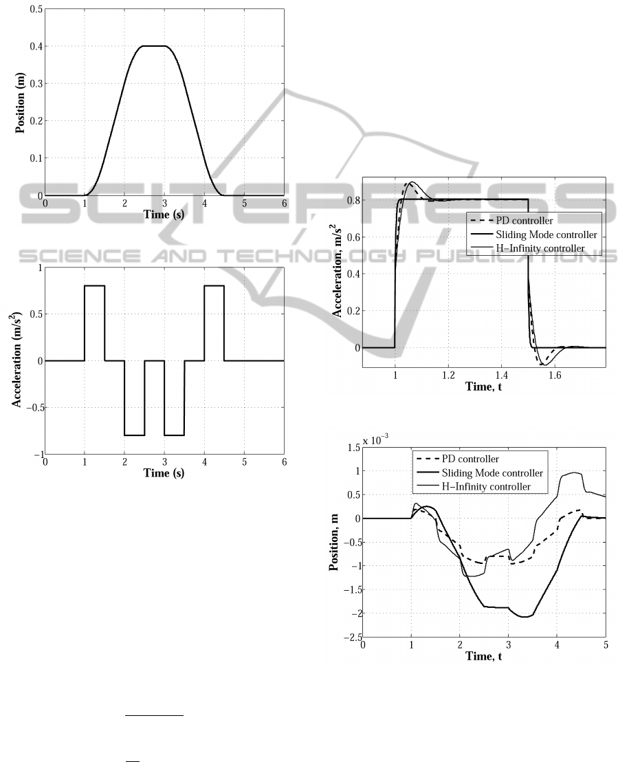
surge (x) and the amplitude of the excitation signals
(step acceleration inputs) was chosen to keep the mo-
tion base approximately 90% of the system limits in
position. Desired position and acceleration are shown
in Fig. 2 and Fig. 3, respectively.
Figure 2: Desired Position - Surge (x).
Figure 3: Desired Acceleration - Surge (x).
The sliding surface parameter ε in Eq. (15) was
chosen as 0.001 (too small values can lead to instabil-
ity problems). The bounding values in Eq. (19) were
calculated by considering exact cancellation in the in-
verse control problem. Thus, Q
M
= 0.8, B
M
= 0.27,
λ = 0.72 and Φ = 23.
On the other hand, in order to yield a low-order H-
Infinity controller, the penalized output signals only
corresponds to the position error and the weighting
functions are given as
W
e
(s) =
s/M
e
+ ω
b
s + ω
b
A
e
;
W
u
(s) =
1
A
u
; W
d
(s) = A
d
(23)
where M
e
= 0.001, A
e
= 1×10
−4
, ω
b
= 100 Hz, A
u
=
10 and A
d
= 6.
With relation to the controller gains in Eq. (7),
(Koekebakker, 2001) state the frequency, ω
i
, should
not exceed human sensory thresholds and that it
should ideally be sufficiently smooth and only re-
quires limited bandwidth (well below 1 Hz).
A bandwidth, ω
i
= 14 Hz and ζ
i
= 0.6 was chosen
to the PD controller (i.e., it is considered the Eq. 6),
ω
i
= 2 Hz and ζ
i
= 5 was chosen to the H-Infinity
controller and ω
i
= 6 Hz and ζ
i
= 1 was chosen to the
sliding mode controller (Eq. (15)).
The step acceleration response and the position er-
ror in surge direction is shown in Fig. 4 and Fig. 5,
respectively. The driving torque of one actuator is
shown in Fig. 6 .
Figure 4: Acceleration response - Surge (x).
Figure 5: Position Error - Surge (x).
From theses figures one can conclude the follow:
∗ The sliding mode controller presented a bigger er-
ror position. As was pointed out above, this tech-
nique not guarantee error convergence to zero, but
ComparisonofRobustControlTechniquesforUseinFlightSimulatorMotionBases
347

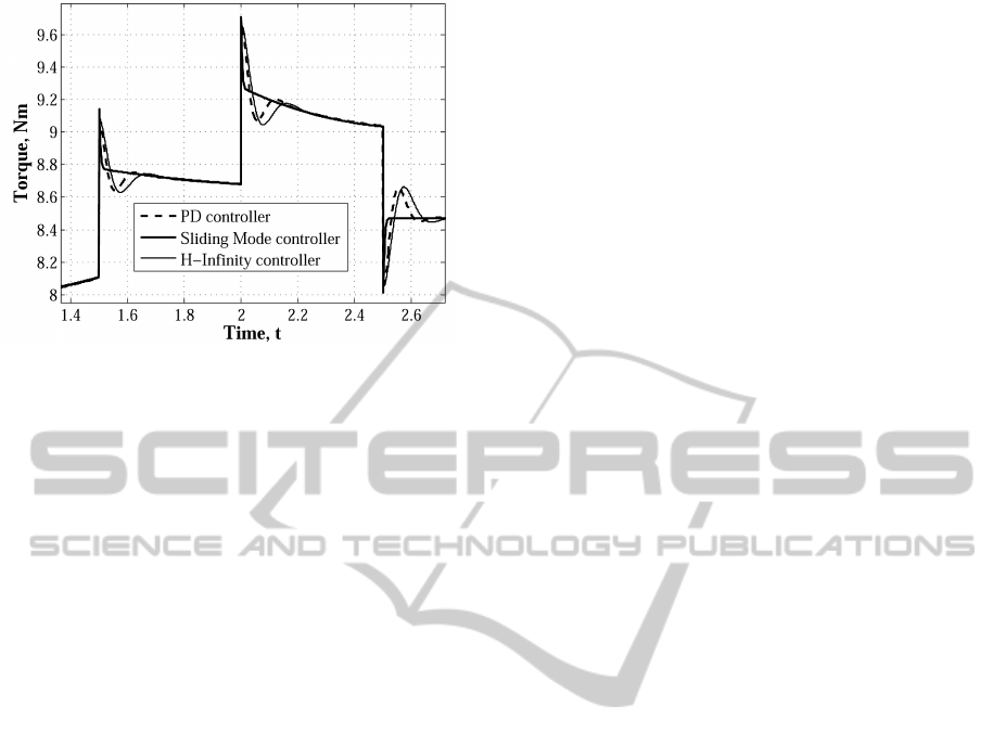
Figure 6: Driving Torque - one actuator.
it ensures bounded-norm error given by ε.
∗ The sliding mode controller presented a rough
motor torque. In this case, the principal contri-
bution to control signal is the u term, therefore
by changing ω
n
and ς won’t affect the response.
By changing P term can be produced a smoother
response. Short time peak torques produce large
jerk and it can lead to false cues.
∗ The inverse dynamic controller without the robust
term got a good response because of high gains in
the controller. High gains can induce instability
and noise amplification. In the other hand, high
gains can produce a rough correction in the accel-
eration and therefore can produce false cues.
∗ The H-Infinity controller presented the smoothest
response but this structure leads an high order
controller.
7 CONCLUSIONS
This article has presented three kinds of control ap-
proaches for the motion control of a flight simula-
tor motion base. All controllers were implemented in
the outer-loop of the inverse dynamic control scheme
in order to counteract imperfect compensation. PD
controller presented a rough response while the other
controllers, i.e, H-infinity and sliding mode controller
presented a smoother response. The reason for that
behaviour is the inclusion of the robust term in the
outer loop of the inverse dynamic control scheme.
There is a tradeoff between the robust term and the
proportional and derivative gains, causing a smooth-
ing or rough response. Future work should be address
practical implementation of these controller .
ACKNOWLEDGEMENTS
The author gratefully acknowledge the financial sup-
port provided by grant 2013/20888-6, S
˜
ao Paulo Re-
search Foundation (FAPESP).
REFERENCES
Becerra-Vargas, M. and Belo, E. (2010). Fuzzy sliding
mode control of a flight simulator motion base. In
27TH Congress of the international Council of the
aeronautical sciences-ICAS 2010, pages 1–12, Nice,
France. Optimage Ltd.
Becerra-Vargas, M. and Belo, E. (2011). Robust control of
a flight simulator motion base. Journal of Guidance,
Control, and Dynamics, 34(5):1519–1528.
Becerra-Vargas, M. and Belo, E. (2012). Application of
H-Infinity theory to a 6 dof flight simulator motion
base. Journal of the Brazilian Society of Mechanical
Sciences and Engineering, 34(2):193–204.
Becerra-Vargas, M. and Belo, E. (2015). Dynamic mod-
eling of a 6 dof flight simulator motion base. Jour-
nal of Computational and Nonlinear Dynamics (doi
10.1115/1.4030013).
Koekebakker, S. (2001). Model based control of a flight
simulator motion system. PhD thesis, Delft University
of Technology, Netherlands.
Sciavicco, L. and Siciliano, B. (2005). Modeling and Con-
trol of Robot Manipulators. Springer-Verlag, Londres,
2 edition.
Spong, M. and Vidyasagar, M. (2006). Robot Modeling and
Control. John Wyley & Sons, New York, 1 edition.
Stewart, D. (1965). A platform with 6 degrees of freedom.
Proceedings of the institution of mechanical engineers
1965-66, 180(15):371–386.
ICINCO2015-12thInternationalConferenceonInformaticsinControl,AutomationandRobotics
348