Stabilizing Global Temperature Through a Fuzzy Control on CO

Emissions

Carlos Gay-Garcia

1,2

and Bernardo Bastien-Olvera

Climate Change Research Program, National University of Mexico, Mexico City, Mexico

Centre for Atmospheric Science, National University of Mexico, Mexico City, Mexico

Keywords:

Climate Change, Global Temperature, Carbon Emissions, Fuzzy Control.

Abstract:

In this research, we generated a fuzzy control of carbon emissions that acts increasing or decreasing the

representative concentration pathway emissions proposed by the IPCC, in order to obtain a CO

path that

would stabilize the global average surface temperature to a desired level. We used a simple linear climate

model that is driven primary by the Carbon emissions. We made simulations under the four RCPs activating

the control at different times, which give us a broad knowledge on when is possible to stabilize the temperature,

based in the current emissions path. We conclude that taking action earlier (via fuzzy control) will lead not

only to reach stabilization, but also, in some cases, to have economic growth allowing to increase emissions

at some points in time. Activating the control very late will initiate an oscillation on temperature which will

include not only a reduction of emissions but also a necessary anthropogenic net carbon sequestration. This

instrument is a common ground where specialists in diverse areas of climate change could contribute in order

to set the parameters that we should explore and simulate so that the we can make the best decisions.

1 INTRODUCTION

The most important Climate Change indicator and

driver is the global average surface temperature which

had already risen by about 0.7

◦

C from pre-industrial

levels. In the United Nations Framework Convention

on Climate Change, COP16, the parties agreed that

the future global warming relative change should be

limited to below 2.0

◦

C (King, 2011).

Since the Cancun agreements, more scientiﬁc

analysis had been done in order to estimate the chance

to constrain the warming, according to Rogelj et al.

(2009) the national emissions targets of developed

countries would need to be adjusted in order to ac-

complish the agreement.

It is very important to identify the windows

of opportunity for action where mitigation cost is

less, Parry and colleagues assumed different emission

peaks and the correspondent percentage of cuts that

would need to be made in order to avoid the most se-

rious global impacts (Parry et al., 2008).

This work is an improved version of a fuzzy con-

trol of emissions that computes the amount of Gt of

increment or decrement that would need to be

made in order to stabilize the temperature to a de-

sired level, using an inference system that evaluates

the closeness of the actual temperature to the target

temperature (Martinez-Lopez and Gay-Garcia, 2011).

Fuzzy controllers had been largely used to achieve

system’s goals in uncertain environments such as

transportation, manufacturing and networked embed-

ded systems (Tong, 1977), furthermore, fuzzy con-

trollers had been implemented to stabilize the climate

on greenhouses (Javadikia et al., 2009), which help

us to sustain our effort of extrapolation to the global

temperature.

2 TEMPERATURE SIMULATION

We used the simple climate model that Tahvonen and

colleagues proposed (Tahvonen et al., 1994) where

the change in atmospheric Carbon concentration (C)

depends on the emission (E) and in the Carbon con-

centration of the system, equation (1). The change

global average surface temperature (T) depends on the

atmospheric Carbon Concentration and on the system

temperature itself, equation (2).

dC(t)

= −σC(t) + βE(t) (1)

526

Gay-Garcia C. and Bastien B..

Stabilizing Global Temperature Through a Fuzzy Control on CO2 Emissions.

DOI: 10.5220/0005547605260531

In Proceedings of the 5th International Conference on Simulation and Modeling Methodologies, Technologies and Applications (MSCCES-2015), pages

526-531

ISBN: 978-989-758-120-5

 2015 SCITEPRESS (Science and Technology Publications, Lda.)

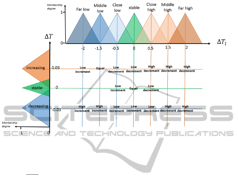
Figure 1: Fuzzy sets and Inference Rules. Top: Closeness to desired temperature, left: change in temperature, inside: change

in carbon emissions. Important note: the fuzzy sets have gaussian shape, the triangules showed here are just used to simplify

the illustration.

dT (t)

= −αT (t) + µC(t) (2)

The constants are σ = 0.018/year, α = 0.03,

µ = 0.00045 (Tahvonen et al., 1994) and β =

0.47ppm/GtC (Maier-Reimer and Hasselman, 1987),

the atmospheric carbon concentration and the global

average surface temperature in the equations are taken

as the anomalies relative to 1959. In our simulations,

the carbon concentration levels (Boden et al., 2013)

and temperature (NASA, 2014) on 2010, are default

settings. The user should set the desired temperature

of stabilization, and the climate model will start com-

puting with the emissions data of one of the Repre-

sentative Concentration Pathways (RCP) (Moss et al.,

2007) that IPCC proposes.

The control input variables are the closeness of the

actual temperature to the target temperature, and the

temperature change, relative to the previous year. The

control output is the change in the carbon emissions

that would need to be made relative to the previous

year emissions in order to drive the temperature to the

desired stabilization level.

Whenever the control is activated, the emissions

will totally depend on the control and the RCP emis-

sions data will no longer be followed.

3 FUZZY CONTROL

The input variables of the fuzzy control are the close-

ness to the desired temperature and the temperature

change relative to the previous year. As it can be seen

in Figure 1, the domain of both variables is divided

into fuzzy sets that follow a linguistic description,

the closeness to temperature domain is divided into

7 fuzzy sets (far low, middle low, close low, desired,

close high, middle high and far high) which represent

how close is the actual temperature to the desired one.

The domain of the temperature change relative to the

previous year is divided into 3 fuzzy sets: increasing,

decreasing, stable.

The control works with inference rules (Figure 1)

that relate the input variables to the change in carbon

emissions that would need to be made, this domain

is divided in 5 fuzzy sets, linguistically described as:

high increment, low increment, equal, low decrement,

high decrement.

The range of action for the input variables was se-

lected having in mind the 2 degrees agreement and the

maximum and minimum change in average tempera-

ture from year to year. The range for the output vari-

able was selected using the maximum and minimum

change in carbon emissions proposed by the IPCC in

the RCPs.

StabilizingGlobalTemperatureThroughaFuzzyControlonCO2Emissions

527

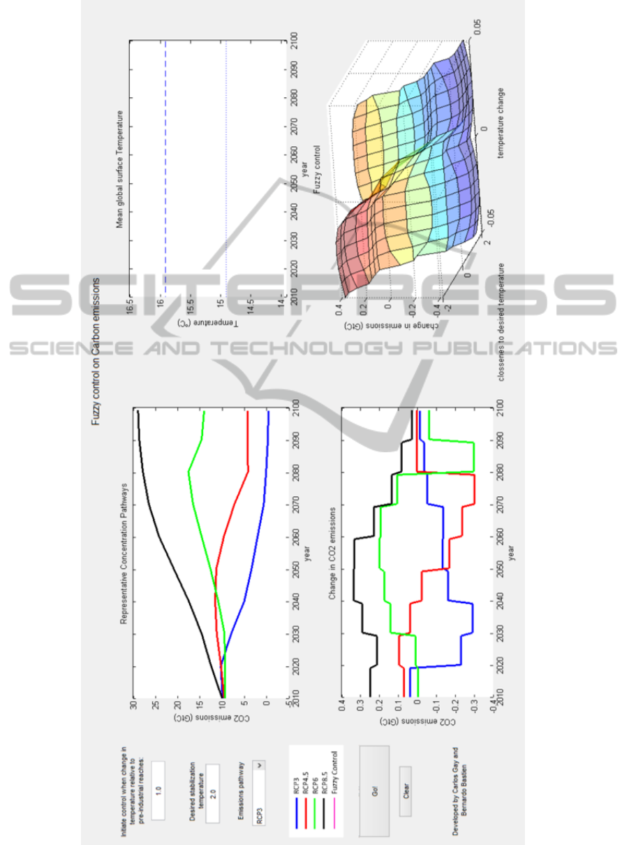
Figure 2: Graphical User interface simulator, more information in Section 4.

SIMULTECH2015-5thInternationalConferenceonSimulationandModelingMethodologies,Technologiesand

Applications

528

4 GRAPHICAL USER

INTERFACE

The principal result of this work is an interactive

Graphical User Interface (GUI) generated in MAT-

LAB (Figure 2) that simulates the temperature and

show the principal results. At the left side there

are three user inputs, the activation temperature, the

desired stabilization temperature and the emissions

pathway that the simulation will follow until the con-

trol is activated.

The top left graphic shows the four possible sce-

narios (RCPs) that the user can choose, the bottom

left panel shows the change in carbon emissions of

those scenarios. At the top right panel are shown

two lines, corresponding to the desired temperature

(dashed line) and the activation temperature (dotted

line). The rules surface, associated to the inference

and rules of the control is shown in the bottom right

side. Whenever the button ”Go” is pushed the simula-

tion will start and a magenta line (or dot) will be draw

on the four graphics, showing the actual path that the

simulation is taking.

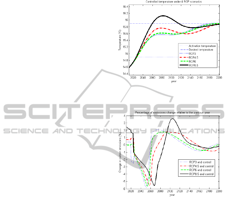
5 EXPERIMENTS

We set the activation temperature at 1

◦

C and the sta-

bilization temperature at 2

◦

C, then we simulate under

the four RCPs and we obtain the results of Figure 3

and 4. As we can see, the temperature paths are quite

different, under RCP3 the stabilization is reached by

the year 2200, and it has a local stabilization from

2050 to 2100. The other projections don’t have any

50-year local stabilization and is not guaranteed the

stabilization at year 2200. Despite of the great differ-

ence on temperature projections, the change in carbon

emissions (%) are very similar, which could indicate

that the actions taken in the incoming years will be

key in the long term global warming.

Furthermore, we ran the model stabilizing at 2

◦

following the four RCPs and activating the control at

◦

C, 1.5

◦

C, 1.8

◦

C and 2

◦

C. The results are shown on

Figure 5.

6 DISCUSSION

6.1 RCP3 Scenario

Following the most optimistic scenario is not the best

option in terms of economic growth and tempera-

ture stabilization, for a few reasons. As we can see

Figure 3: Temperature projected under the RCP scenar-

ios, until activation temperature is reached (1

◦

C from pre-

industrial. Stabilization temperature: 2

◦

C. Activation year:

2026 for RCP3,

Figure 4: Percentage of emissions that would need to

change relative to the previous year.

in Figure 5: Row1, Column1 (R1C1), the emissions

control that activates at 1

◦

C and 1.5

◦

C stabilize the

temperature at 2

◦

C (15.9

◦

C) and in R1C2 is shown

that an earlier control lead to emit more carbon than

the suggested by the scenario. The activation tem-

peratures set in 1.8

◦

C and 2

◦

C do not ﬁre the con-

trol because under the RCP3 scenario the temperature

never reaches those numbers, in R1C2 we can see that

the change in carbon emissions relative to the previ-

ous year is vertical for those activation temperatures,

this is because the change in emissions indeterminate,

which means that the emissions cross the zero and

carbon sequestration is supposed.

6.2 RCP4.5 Scenario

In R2C1 is shown that all temperatures could reach

stabilization but an early control activation avoids

StabilizingGlobalTemperatureThroughaFuzzyControlonCO2Emissions

529

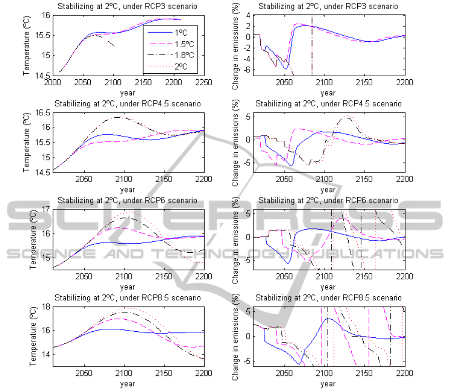
Figure 5: Simulations under RCP3, RCP4.5, RCP6 and RCP8. The control is activated at 1

◦

C, 1.5

◦

C, 1.8

◦

C and 2

◦

C, each

row of plots represents an RCP (R1:RCP3 and so on). The ﬁrst column (C1) is for temperature and the second column (C2)

is for their respective change in emissions

temperature overshooting. We can also observe in

R2C2 that an earlier activation the negative peak is

reached earlier but the amplitude between the neg-

ative and the positive peaks is less, which means

that technologies and global policies wouldn’t have

to change drastically in a few years.

6.3 RCP6 Scenario

In R3C2 of Figure 5, is shown that the temperture sta-

bilization is reached only when the control is activated

at 1

◦

C and 1.5

◦

C (with overshooting), otherwise dur-

ing the ﬁrst 200 years the temperature will acquire an

oscillatory behaviour, moreover in R3C2 we can see

that activating the control at 1.8

◦

C and 2

◦

C would im-

ply carbon sequestration methods.

6.4 RCP8.5 Scenario

If the emissions path follow the worst scenario in

the following years, a temperature stabilization (with

overshooting) could be reached only if the control

activates very early, at 1

◦

C (R4C1). Otherwise the

temperature would oscillate and carbon sequestration

would be needed (R4C2).

7 CONCLUSIONS

With the results obtained in the simulations we can

take decisions by answering the following question:

Under which scenario we are developing? So then, it

is possible to observe at what temperature we should

SIMULTECH2015-5thInternationalConferenceonSimulationandModelingMethodologies,Technologiesand

Applications

530

activate the control in order to stabilize the temper-

ature. There are some cases where the control acti-

vation leads to increment the emissions immediately,

which can give us an idea that this kind of control can

also lead to economic growth.

This simulation tool with the fuzzy control pro-

posed is a very powerful instrument in climate change

policy and international agreements. The conﬁgura-

tion options allow us to project under certain circum-

stances that answer the questions: When are we tak-

ing action? and, What is our goal stabilization tem-

perature?

The results will give us not just how many GtC

we should decrease or increase every year, but also

the percentage of emissions relative to the previous

year, which could give us an idea of how much it will

cost us (Figure 4).

This instrument is a common ground where spe-

cialists in diverse areas of climate change could con-

tribute in order to set the parameters that we should

explore and simulate so that the we can make the best

decisions.

In future work, we seek to not only project the

amount of carbon emissions that should be changed,

but also the amount which each country should con-

tribute to accomplish the goal, based on a fuzzy infer-

ence system that asses every country possibilities ans

responsibility.

REFERENCES

Boden, T. A., Marland, G., and Andres, R. J. (2013).

Global, regional, and national fossil-fuel co2 emis-

sions.

Javadikia, P., Tabatabaeefar, A., Omid, M., Alimardani, R.,

and Fathi, M. (2009). Evaluation of intelligent green-

house climate control system, based fuzzy logic in

relation to conventional systems. In Artiﬁcial Intel-

ligence and Computational Intelligence, 2009. AICI

’09. International Conference on, volume 4, pages

146–150.

King, D. (2011). ”copnhagen and cancun”, internationl cli-

mate change negotiations: Key lessons and next steps.

Smith School of Enterpise and the Environment, Uni-

versity of Oxford, :12.

Maier-Reimer, E. and Hasselman, K. (1987). Transport

and storage of co2 in the ocean - an inorganic ocean-

circulation carbon cycle model. Clim Dynam, (2):63–

90.

Martinez-Lopez, B. and Gay-Garcia, C. (2011). Fuzzy con-

trol of co2 emissions. Proceedings: Eigth Interna-

tional Conference on Fuzzy Systems and Knowledge

Discovery.

Moss, R., Babiker, M., Brinkman, S., Calvo, E., Carter, T.,

Edmonds, J., Elgizouli, I., Emori, S., Erda, L., Hib-

bard, K., Roger, J., Kainuma, M., Kelleher, J., Lamar-

que, J. F., Manning, M., Matthews, B., Meehl, J.,

Meyer, L., Mitchell, J., Nakicenovik, N., O’Neill, B.,

Pichs, R., Riahi, K., Rose, S., Runc, P., Stouffer, R.,

van Vuuren, D., Weyant, J., Wilbanks, T., van Yper-

sele, J. P., and Zurek, M. (2007). Towards new scenar-

ios for analysis of emissions, climate change, impacts,

and response strategies. IPCC Expert meeting report.

NASA (2014). Giss surface temperature analysis (gistemp).

giss.nasa.gov.

Parry, N., Palutikof, J., Hanson, C., and Lowe, J. (2008).

Squaring up to reality. Nature Reports Climate

Change, :68–71.

Tahvonen, O., Von Storch, H., and Von Storch, J. (1994).

Economic efﬁcency of co2 reduction programs. Clim

Res, (4):127–141.

Tong, R. (1977). A control engineering review of fuzzy

systems. Automatica, 13(6):559 – 569.

StabilizingGlobalTemperatureThroughaFuzzyControlonCO2Emissions

531