Unconstrained Global Optimization: A Benchmark Comparison of

Population-based Algorithms

Maxim Sidorov

, Eugene Semenkin

and Wolfgang Minker

Institute of Communication Engineering, Ulm University, Ulm, Germany

Institute of System Analysis, Siberian State Aerospace University, Krasnoyarsk, Russia

Keywords:

Genetic Algorithm, Evolution Strategy, Cuckoo Search, Differential Evolution, Particle Swarm Optimization,

Benchmark Comparison, Unconstrained Optimization.

Abstract:

In this paper we provide a systematic comparison of the following population-based optimization techniques:

Genetic Algorithm (GA), Evolution Strategy (ES), Cuckoo Search (CS), Differential Evolution (DE), and

Particle Swarm Optimization (PSO). The considered techniques have been implemented and evaluated on a

set of 67 multivariate functions. We carefully selected the tested optimization functions which have different

features and gave exactly the same number of objective function evaluations for all of the algorithms. This

study has revealed that the DE algorithm is preferable in the majority of cases of the tested functions. The

results of numerical evaluations and parameter optimization are presented in this paper.

1 INTRODUCTION

Evolutionary and behavioural algorithms such as GA,

ES, PSO, CS, and DE have recently been success-

fully applied to a wide variety of problems includ-

ing machine learning, multi-modal function optimiza-

tion, the evolution of complex structures such as ar-

tiﬁcial neural networks or even computer programs.

However, one of the most signiﬁcant weaknesses of

these algorithms is the necessity of setting the opti-

mal parameters and selecting the suitable algorithm in

each speciﬁc real-world problem. Moreover, it could

be difﬁcult to optimize high-dimensional, multivari-

ate functions using the mentioned algorithms due to a

large number of local extrema, the surface of a com-

plex function, etc.

In this paper we performed a comparative study

where we dealt with the most popular population-

based algorithms. In order to fairly compare the con-

sidered algorithms we performed an optimization pro-

cess using 67 functions which are considered to be

difﬁcult for optimization. We gave the same number

of function evaluations for all the algorithms and car-

ried out an optimization of the parameters for all of

the algorithms. To enhance the statistical reliability

of the experiments we repeated the process of func-

tion optimization 100 times with each combination of

parameters. The study revealed that the DE algorithm

was generally found to perform better than other al-

gorithms.

The rest of the paper is organized as follows: Sig-

niﬁcant related work is presented in Section 2. We

brieﬂy describe the used algorithms in Section 3. Fur-

ther, the set up of the experiments, their results, and

the used functions are in Section 4. Finally, Section 5

presents the conclusion and future work.

2 SIGNIFICANT RELATED

WORK

The comparison of the population-based optimization

algorithms is a focus of scientiﬁc groups all over the

world.

Thus, the authors in (Eberhart and Shi, 1998)

compared the PSO algorithm with GA in a theoretical

way. In this paper the individual features of the algo-

rithms were highlighted, moreover the authors noted

that the performance of one algorithm might be im-

proved by incorporating features of the other.

In (Elbeltagi et al., 2005) a comparison of ﬁve

evolutionary-based optimization algorithms was pre-

sented. The authors researched the following algo-

rithms: GA, memetic algorithms, PSO, Ant-Colony

Optimization, and the Shufﬂed Frog Leaping Al-

gorithm. Two benchmark continuous optimization

test problems were solved using the considered algo-

230

Sidorov M., Semenkin E. and Minker W..

Unconstrained Global Optimization: A Benchmark Comparison of Population-based Algorithms.

DOI: 10.5220/0005548002300237

In Proceedings of the 12th International Conference on Informatics in Control, Automation and Robotics (ICINCO-2015), pages 230-237

ISBN: 978-989-758-122-9

 2015 SCITEPRESS (Science and Technology Publications, Lda.)

rithms. The authors concluded that the PSO method

was generally found to perform better than other al-

gorithms. Among some weaknesses of the study one

may note that only two test functions could not give

statistical reliable results.

3 OPTIMIZATION ALGORITHMS

OF DIRECT SEARCH

In this section we present a brief description of the

used algorithms. Suppose that the given objective

function is f (x), where x = (x

, ..., x

3.1 Cuckoo Search

CS is a population-based optimization method devel-

oped in (Yang and Deb, 2009) which imitates the be-

haviour of cuckoos in their natural habitats utilizing

the concept of Levy ﬂight. Cuckoos lay their eggs in

other birds’ nests and rely on other birds to raise their

offspring. It is believed that such selﬁsh behaviour in-

creases the survival rate of the cuckoo’s genes since

the cuckoo needs not spend any energy and time rais-

ing its offspring. Thus, the time and energy saved

can be used by the cuckoo in order to breed and lay

more eggs (Lidberg, 2011). Nevertheless, there exist

special strategies which allow the birds to detect the

invading eggs. The CS algorithm uses this behaviour

to traverse the search space, looking for the optimal

solution. CS consists of the following stages:

Step 1. Initialization

A pool of initial solutions should better cover the

whole search space by uniformly randomizing within

the area which is constrained by the given lower and

upper boundaries. Practically, each j −th component

of the initial i −th solution is formed in conformity

with the following equation:

i,0

= x

min

+ r(0, 1) ×(x

max

−x

min

) , (1)

where, x

max

and x

min

are the corresponding bound-

aries of the j −th variable, and r(0, 1) is a uniformly

distributed random variable from [0, 1]. Then, initial

solutions should be evaluated in order to obtain the

current best.

Step 2. Generate a Solution by Levy Flights

After the initialization and the ﬁrst assessment steps,

new solutions should be generated by Levy walk

around the best solution obtained so far:

= x

i−1

+ N(0,1) ×

0.01 ×



σ ×N(0.1)

|N(0,1)|

×(x

i−1

−x

best

)



where

σ =





Γ(1 + β)sin



πβ





1+β



β2

(β−1)





Γ(z) is gamma function, 1 ≤ β ≤ 2, N(0, 1) is a nor-

mal distributed n-dimensional vector with µ = 0 and

= 1, x

and x

i−1

are the current and previous solu-

tions, x

best

is the best solution found so far, and all the

operations with vectors are element-based.

Step 3. Evaluate Quality of Solutions

At this point all the new solutions should be evaluated

and in case of improvement in the value of the objec-

tive function, the old solution should be replaced by

the new one.

Step 4. Discovery and Randomization

Now, new solutions should be discovered with the

given probability pa:

(

i−1

, if r(0, 1) < pa

i−1

×r(0, 1) ×(x

−x

), otherwise.

where x

and x

are randomly chosen different solu-

tions, they must be distinct from each other, and pa is

the discovery rate of alien solutions (or eggs).

Step 5. Rank the Solutions

Here all the current solutions should be ranked and

the global best is saved.

The Steps 2 to 5 are repeated until the stop cri-

terion is True. Only two parameters should be sup-

plied to the algorithm, the discovery rate of alien eggs

pa ∈[0, 1] and the size of population. Pa plays an im-

portant role controlling the elitism and the trade-off

between randomization and local search (Yang and

Deb, 2010). In this study we used the grid technique

for optimization of the pa parameter form [0, 1] with

the step equal to 0.1, and only two values for the size

of population, namely 25 and

√

bud, where bud is the

number of objective function evaluations.

3.2 Differential Evolution

DE is a simple yet powerful evolution algorithm for

unconstrained global optimization introduced and dis-

cussed in (Storn and Price, 1995), (Storn and Price,

1997), and (Price et al., 2006). CS consists of the fol-

lowing stages:

UnconstrainedGlobalOptimization:ABenchmarkComparisonofPopulation-basedAlgorithms

231

Step 1. Initialization

This step should be done in a similar to way how it

was done in the case of CS (see Equation 1).

Step 2. Compute the Potentially New Position

Further, depending on the selected strategy apply the

following formula in order to get a new solution x

i, j

DE/rand/1

i, j

= x

i−1,c

+ w ×(x

i−1,a

−x

i−1,b

) ,

DE/local-to-best/1

i, j

= x

i−1, j

+ w ×(x

i−1,best

−x

i−1, j

)

+ w ×(x

i−1,a

−x

i−1,b

) ,

DE/best/1 with jitter

i, j

= x

i−1,best

+ (x

i−1,a

−x

i−1,b

)

×(0.001 ×r(0, 1) + w) ,

DE/rand/1 with per-vector-dither

i, j

= x

i−1,c

+ (x

i−1,a

−x

i−1,b

)

×(1 −w) ×r(0, 1) + w ,

DE/rand/1 with per-generation-dither

i, j

= x

i−1,c

+ (x

i−1,a

−x

i−1,b

)

×(1 −w) ×r(0, 1) + w ,

Either-or-algorithm

i, j











i−1,c

+ w ×(x

i−1,a

−x

i−1,b

), ifr(0, 1) < 0.5

i−1,c

+ 0.5 ×(w + 1)

×(x

i−1,a

+ x

i−1,b

−2x

i−1,c

) , otherwise.

where x

i−1,a

, x

i−1,b

, and x

i−1,c

are three randomly

picked solutions from the previous iteration, they

must be distinct from each other. Practically, it can

be done by a random solution permutation within the

whole population. x

i−1,best

is the best solution from

the previous iteration, w is the step size, usually from

[0, 2].

Step 3. Crossover

Next, the obtained solutions should be placed in the

next generation with the given crossover probability

cr.

i, j

(

i, j−1

, ifr(0, 1) <cr

i, j

, otherwise.

Step 4. Rank the Solutions

Here all the current solutions should be ranked and

the global best is saved.

The Steps 2 to 4 should be repeated until the stop

criterion is True.The choice of DE parameters cr, w,

the number of solutions in each generation and the

new solution generation strategy can have a large im-

pact on optimization performance. In this study we

used all types of strategies, as well as cr and w param-

eters from [0,1] with the step equal to 0.1. A constant

number of solutions in each generation has been set

√

bud.

3.3 Evolution Strategy

The ES which was proposed by Schwefel, and

Rechenberg (Beyer and Schwefel, 2002) operates

with real numbers directly. We implemented the ES

algorithm based on (Haupt and Haupt, 2004) and

(Back, 1996). The ES comprises the following steps:

Step 1. Initialization

This step should be done in a similar way to how it

was done in the case of CS and DE (see Equation 1).

Step 2. Recombination

Further, depending on the selected recombination

strategy apply the following formula in order to get

a new solution x

i, j

and the corresponding parameters

i, j

and α

i, j

No recombination

i, j

= x

i−1,r(1,µ)

where j = 1...λ, and r(1, µ) is a uniform distributed

random variable from [1, µ].

Discrete recombination

This type of recombination determines the k−th com-

ponent of the recombinant exclusively by the k −th

component of the randomly (uniformly) chosen two

parent individuals (Beyer and Schwefel, 2002):

i, j,k

= x

i−1,r(1,µ),k

Panmictic discrete recombination

The same as above, but in this case more than two

parents can be selected in order to produce the cur-

rent offspring.

Intermediate recombination

Intermediate recombination calculates the average

values of the corresponding components of the two

parent vectors.

Panmictic intermediate recombination

Again, the same as the previous one, but in this case

more than two parents can be selected in order to pro-

duce the current offspring.

Generalized intermediate recombination

i, j

= x

i−1,a

+ r(0, 1) ×(x

i−1,b

−x

i−1,a

), (2)

where x

i−1,a

, x

i−1,b

are randomly selected solutions

from the previous generation, r(0, 1) is as usually a

uniform distributed variable from [0, 1].

Generalized intermediate recombination

ICINCO2015-12thInternationalConferenceonInformaticsinControl,AutomationandRobotics

232

The same as the previous one, but now more than two

parents can be selected in order to produce the current

offspring using Equation 2.

In order to simplify a description of the algorithm,

only solution-based formulas have been displayed, it

should be noted that the corresponding parameters

i, j

and α

i, j

are converted in exactly the same way

as was done for the position variables.

Step 3. Mutation

Mutation is used to ensure the evolutionary diversity

and has been implemented using Equation 2.18 from

(Back, 1996).

Step 4. Selection

In this study we used the standard (µ, λ)and(µ + λ)

selection types.

Step 5. Rank the Solutions

Here all the current solutions should be ranked and

the global best is saved.

The Steps 2 to 5 should be repeated until the stop cri-

terion is True. Regarding the parameters of the ES

procedure, we tried all types of recombination for so-

lutions and parameters independently. The last pa-

rameter is the type of selection.

3.4 Genetic Algorithm

GA, which was originally conceived by Holland (Hol-

land, 1975), represents an abstract model of Dar-

winian evolution where a candidate solution (or indi-

vidual) is encoded with the boolean values (or genes).

In case of pseudo-boolean GA, each gene is ﬁlled

with boolean true with the probability equal to 0.5 and

with false otherwise. Let Lower and Upper be the cor-

responding boundaries of the search space and Accu-

racy be the desirable accuracy of the optimal solution.

Then, the necessary number of bits for encoding (N)

is equal to the lowest value for which the following

equation is true:

≥

U pper −Lower

0.1 ×Accuracy + 1

, (3)

thus, each GA’s individual is (n × N)-dimensional

boolean vector, where n is the number of variables

in the optimization task.

A pool of initial individuals (or population) should

better cover the whole search space by uniformly ran-

domizing within the area which is constrained by the

given lower and upper boundaries. Practically, each

gene is ﬁlled with boolean true with the probability

equal to 0.5 and with false otherwise.

The next phase is assessment of each solution.

For this reason, each Boolean vector should be de-

coded to an integer vector either with the conventional

boolean-to-integer encoding scheme or with Gray

coding (Gray, 1953). Lastly, to produce the real val-

ues the corresponding interval from [Lower,U pper]

should be selected. The resulting real vector is used

to obtain the current value of the objective function.

Intuitively, the lower the value of the objective

function, the higher the probability that there is a

corresponding individual. For this reason, the selec-

tion procedure should be applied in order to enhance

the probability of including the perspective candidates

into the next generation of GA. We used three differ-

ent strategies of the selection procedure. Proportional

and rank selections operate with the absolute and rank

values of current solutions respectively. It means that

the higher the ﬁtness value or corresponding rank,

which can be obtained by the sorting procedure, the

higher the probability that it is selected. Whereas in

tournament selection, the individual with the higher

ﬁtness function from the group with n individual is

selected into the next generation. The recombination

procedure provides the similarity of the individuals in

the next generation to the best individuals from the

previous one. Lastly, mutation supports the evolution

diversity of individuals.

The described procedure is repeated until the ter-

minate condition is true.

We optimized all the parameters: accuracy,

elitism, Gray coding, types of mutation, selection and

recombination.

3.5 Particle Swarm Optimization

Being a behavioural algorithm, the PSO technique

(Kennedy et al., 1995) simulates the behaviour of ani-

mal swarms in their natural habitats. The algorithm

optimizes a function by having a number of solu-

tions or particles and moving these particles within

the search-space according to the mathematical for-

mulas. Each particle is characterised by position and

velocity values. The movement of a particular solu-

tion within the search-space is inﬂuenced by its local

best known position and the global best known posi-

tion in the search-space, which was achieved by other

particles. More precisely, the following formulas de-

termine the velocity and position of each particle dur-

ing the algorithm ﬂow:

i,d

= wv

i,d

+ c

i,d

−x

i,d

) + c

−x

i,d

) , (4)

= x

+ v

, (5)

where v

i,d

is the d −th velocity component of the i −

th particle, p

i,d

is the d −th local best element of the

i −th particle, g

is the d −th global best component

of the i −th particle. r

and r

are normal-distributed

UnconstrainedGlobalOptimization:ABenchmarkComparisonofPopulation-basedAlgorithms

233

variables with mean equal to 0 and variance equal to

1, while w, c

and c

are parameters of the algorithm

to be optimized.

Moreover, an absolute value of the velocity is al-

ways limited by the VelocityMax. In our implementa-

tion this parameter was determined by the following

formula:

VelocityMax = k

(U pper −Lower)

where U pper and Lower are the corresponding

boundaries of the search-space, k is the fourth param-

eter to be optimized.

All the described algorithms have been tested us-

ing 67 test functions with different features and di-

mensionalities.

4 THE USED APPROACH

All the considered algorithms were implemented

from scratch on C++ language using the Boost library.

We adopted the MVF Library (Adorio and Diliman,

2005) to deal with the benchmark test function.

There are a number of standard functions (Adorio

and Diliman, 2005) which have different features and

are difﬁcult to optimize. The community uses such

functions to examine the optimization ability of de-

veloped algorithms.

The suggested baseline implementation of GA,

ES, CS, DE and PSO has been tested on 67 multi-

variate functions for unconstrained global optimiza-

tion. The selected functions are listed in Table 2,

where Opt. and D. stand for the optimal value and the

function dimensionality correspondingly. It should be

noted that the corresponding formulas can be found

here (Adorio and Diliman, 2005).

Some functions can be characterized in the follow-

ing way.

Many Local Minima. The Ackly function is char-

acterized by a nearly ﬂat outer region, and a large

hole at the centre. The function poses a risk for

optimization algorithms of being trapped in one of

its many local minima. The Griewank function has

many widespread local minima, which are regularly

distributed. The Rastrigin function has several local

minima. It is highly multi-modal, but the locations of

the minima are regularly distributed.

Bowl-shaped. The Bohachevsky functions are

slightly different but all of them have the same similar

bowl shape. The Sphere function has 2 local minima

in addition to the global one. It is continuous, con-

vex and unimodal. The Sum Squares function, also

referred to as the Axis Parallel Hyper-Ellipsoid func-

tion, has no local minimum except the global one.

Plate-shaped. The Booth function is plate-

shaped. The Matyas and Zakharov functions have no

local minima except the global one.

Valley-shaped. The Rosenbrock function is re-

ferred to as the Valley or Banana function, and is a

popular test problem for gradient-based optimization

algorithms. The function is unimodal, and the global

minimum lies in a narrow, parabolic valley. However,

even though this valley is easy to ﬁnd, convergence to

the minimum is difﬁcult.

In fact, the efﬁciency of an optimization algorithm

highly depends on its parameters, therefore the pa-

rameters of standard algorithms have been optimized

with the brute force approach using the grid tech-

nique. The optimized parameters and their potential

values can be found in Table 1.

Table 1: Parameters optimization setup, with the abbrevia-

tions of parameters in parentheses.

Parameter Values

pa [0.1, 0.2, ..., 1.0]

Crossover probabil-

ity (CR)

[0, 0.1, ..., 1.0]

Stepsize weight (W) [0, 0.1, ..., 1.0]

Strategy (S) rand/1, local-to-best/1, best/1 with

jitter, rand/1 with per-vector-dither,

rand/1 with per-generation-dither,

rand/1 either-or-algorithm

Variable Recombi-

nation (VR)

Without, discrete, panmictic discrete,

intermediate, panmictic intermediate,

generalized intermediate, panmictic

generalized intermediate

Parameter Recombi-

nation (PR)

The same as above

Selection (P) (µ, λ), (µ + λ)

Gray (G) false, true

Elitism (E) false, true

Selection (S) proportional, rank, tournament

Recombination (R) one-, two-points, uniform

Mutation (M) weak, normal, strong

Accuracy (A) [0.001, 0.0001]

Tournament (T) [2, 3, ..., 5]

PSO

[1.5, 1.6, ..., 1.9]

k [0.1, 0.3, ..., 0.9]

w [0.8, 0.9, ..., 1.1]

ICINCO2015-12thInternationalConferenceonInformaticsinControl,AutomationandRobotics

234

Table 2: The used function and their description. D. stands for dimensionality, Lower, Upper are the corresponding boundaries

of the search-space, and Opt. is an optimal value of the function.

Function D. Lower Upper Opt. Function D. Lower Upper Opt.

Ackley 2 -32.768 32.768 0 NeumaierPerm0 2 -1 1 0

Beale 2 -4.5 4.5 0 NeumaierPowersum 2 0 4 0

Bohachevsky1 2 -100 100 0 NeumaierTrid 2 -4 4 -2

Bohachevsky2 2 -100 100 0 Paviani 2 0.001 9.999 -45.778

Booth 2 -10 10 0 QuarticNoiseU 2 -1.28 1.28 0

BoxBetts 3 0.9 11.2 0 QuarticNoiseZ 2 -1.28 1.28 differ

Branin 2 -5 15 0.398 Rastrigin 2 -5.12 5.12 0

Branin2 2 -5 15 0 Rastrigin2 2 -5.12 5.12 0

Camel6 2 -5 5 -1.032 Rosenbrock 2 -10 10 0

Cola 17 -4 4 11.746 Schaffer1 2 -100 100 0

Colville 4 -10 10 0 Schaffer2 2 -100 100 0

Corana 4 -1000 1000 0 Schwefel1 2 2 -10 10 0

Easom 2 -100 100 -1 Schwefel2 21 2 -10 10 0

Exp2 2 0 20 0 Schwefel2 22 2 -10 10 0

FraudensteinRoth 2 -20 20 0 Schwefel2 26 2 -500 500 -12569.5

Gear 4 12 60 0 Shekel10 10 0 10 0

GeneralizedRosenbrock 2 -10 10 0 Shekel4 10 4 0 10 -10.536

GoldsteinPrice 2 -2 2 3 Shekel4 5 4 0 10 -10.153

Griewank 2 -100 100 0 Shekel4 7 4 0 10 -10.403

Hansen 2 -10 10 -176.54 Shubert 2 -10 10 -24.063

Hartman3 3 0 1 -3.86 Shubert2 2 -10 10 -186.731

Hartman6 6 0 1 -3.32 Shubert3 2 -10 10 -24.063

Himmelblau 2 -5 5 0 Sphere 2 -10 10 0

Holzman2 2 -10 10 0 Sphere2 2 -10 10 0

Hyperellipsoid 2 -1 1 1 Step 2 -100 100 0

Kowalik 4 -5 5 0 StretchedV 2 -10 10 0

Langerman 2 0 10 -1.4 SumSquares 2 -10 10 0

Leon 2 -10 10 0 Trecanni 2 -5 5 0

Matyas 2 -10 10 0 Trefethen4 2 -6.5 6.5 -3.307

Maxmod 2 -10 10 0 Watson 6 -10 10 0.002

McCormick 2 -3 4 -1.913 Xor 9 -10 10 0

Michalewitz 2 0 π -1.932 Zettl 2 -10 10 -0.004

Multimod 2 -10 10 0 Zimmerman 2 -100 100 0

NeumaierPerm 2 -2 2 0

We applied the grid optimization scheme in order

to ﬁnd out the best parameters of each algorithm and

test function. For every combination of the optimized

parameters we repeated the optimization process 100

times to obtain statistical signiﬁcant results. We gave

the same number of objective function evaluations for

all the algorithms. Namely, Num = 100 ×n

, where n

is the dimensionality of the test function.

The results of test function optimization with the

optimal parameters of algorithms is in Figure 1 where

only average (over 100 algorithm runs) values are

shown. The best values are highlighted with darker

colours. The lower the value, the darker the corre-

sponding cell.

5 CONCLUSIONS

Regarding the results of standard algorithm applica-

tions one may conclude that DE is the best algorithm.

The optimal parameters were a wide variety of all

possible settings. However, CR equal to 0.1, W to

0.6 and the rand/1 either-or strategy seem to be an

optimal choice for majority of the functions. Never-

theless, for some optimization functions DE was out-

performed by GA and PSO (see Figure 1).

It should be noted that in the case of GA the tour-

nament selection as well as the (µ + λ) selection for

ES were always selected as the optimal choice for all

of the functions.

One of the possible further directions of investi-

gation might be the usage of a cooperative scheme,

where each algorithm might use the features of oth-

ers in order to improve the performance as was done

here (Sidorov et al., 2014b) for GA, ES and PSO

only and in (Akhmedova and Semenkin, 2013) for

PSO-like algorithms. Moreover, an implementation

of the self-adaptive operators for evolution algorithms

(Sidorov et al., 2014a), (Semenkin and Semenkina,

2012) could signiﬁcantly simplify the process of set-

UnconstrainedGlobalOptimization:ABenchmarkComparisonofPopulation-basedAlgorithms

235

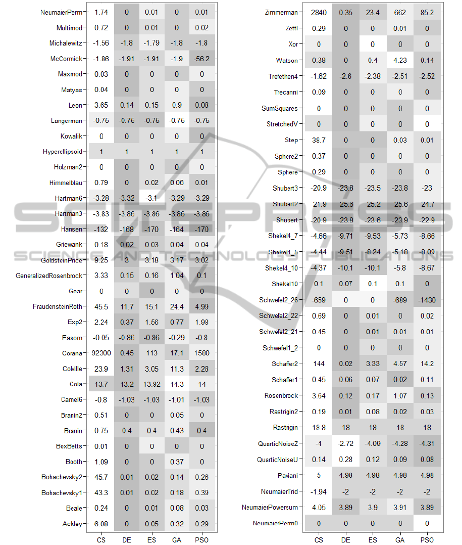
Figure 1: Means of the minimum values over 100 runs of the corresponding algorithm with all possible combinations of

the considered parameters. The darker cell, the better solution was found with the optimal parameters of the corresponding

algorithm. The best values are highlighted with gray colour, the worst ones are coloured with white colour.

ting parameters. Such algorithms could also be in-

cluded in cooperative schemes.

REFERENCES

Adorio, E. P. and Diliman, U. (2005). Mvf-multivariate test

functions library in c for unconstrained global opti-

ICINCO2015-12thInternationalConferenceonInformaticsinControl,AutomationandRobotics

236

mization.

Akhmedova, S. and Semenkin, E. (2013). Co-operation of

biology related algorithms. In Evolutionary Compu-

tation (CEC), 2013 IEEE Congress on, pages 2207–

2214. IEEE.

Back, T. (1996). Evolutionary algorithms in theory and

practice. Oxford Univ. Press.

Beyer, H.-G. and Schwefel, H.-P. (2002). Evolution

strategies–a comprehensive introduction. Natural

computing, 1(1):3–52.

Eberhart, R. C. and Shi, Y. (1998). Comparison between

genetic algorithms and particle swarm optimization.

In Evolutionary Programming VII, pages 611–616.

Springer.

Elbeltagi, E., Hegazy, T., and Grierson, D. (2005).

Comparison among ﬁve evolutionary-based optimiza-

tion algorithms. Advanced engineering informatics,

19(1):43–53.

Gray, F. (1953). Pulse code communication. US Patent

2,632,058.

Haupt, R. L. and Haupt, S. E. (2004). Practical genetic

algorithms. John Wiley & Sons.

Holland, J. H. (1975). Adaptation in natural and artiﬁcial

systems: An introductory analysis with applications to

biology, control, and artiﬁcial intelligence. U Michi-

gan Press.

Kennedy, J., Eberhart, R., et al. (1995). Particle swarm op-

timization. In Proceedings of IEEE international con-

ference on neural networks, volume 4, pages 1942–

1948. Perth, Australia.

Lidberg, S. (2011). Evolving cuckoo search: From single-

objective to multi-objective.

Price, K., Storn, R. M., and Lampinen, J. A. (2006). Differ-

ential evolution: a practical approach to global opti-

mization. Springer Science & Business Media.

Semenkin, E. and Semenkina, M. (2012). Self-conﬁguring

genetic algorithm with modiﬁed uniform crossover

operator. In Advances in Swarm Intelligence, pages

414–421. Springer.

Sidorov, M., Brester, K., Minker, W., and Semenkin, E.

(2014a). Speech-based emotion recognition: Feature

selection by self-adaptive multi-criteria genetic algo-

rithm. In International Conference on Language Re-

sources and Evaluation (LREC).

Sidorov, M., Semenkin, E., and Minker, W. (2014b). Multi-

agent cooperative algorithms of global optimization.

In Proceedings of the 11th International Conference

on Informatics in Control, Automation and Robotics

(ICINCO), volume 1, pages 259–265.

Storn, R. and Price, K. (1995). Differential evolution-a sim-

ple and efﬁcient adaptive scheme for global optimiza-

tion over continuous spaces, volume 3. ICSI Berkeley.

Storn, R. and Price, K. (1997). Differential evolution–a

simple and efﬁcient heuristic for global optimization

over continuous spaces. Journal of global optimiza-

tion, 11(4):341–359.

Yang, X.-S. and Deb, S. (2009). Cuckoo search via l

evy

ﬂights. In Nature & Biologically Inspired Computing,

2009. NaBIC 2009. World Congress on, pages 210–

214. IEEE.

Yang, X.-S. and Deb, S. (2010). Engineering optimi-

sation by cuckoo search. International Journal of

Mathematical Modelling and Numerical Optimisa-

tion, 1(4):330–343.

UnconstrainedGlobalOptimization:ABenchmarkComparisonofPopulation-basedAlgorithms

237