Neural Modeling and Control of a
13
C Isotope Separation Process
Vlad Muresan
1
, Mihail Abrudean
1
Honoriu Valean
1
, Tiberiu Colosi
1
, Mihaela-Ligia Ungureşan
2
,
Valentin Sita
1
, Iulia Clitan
1
and Daniel Moga
1
1
Automation Department, Technical University of Cluj-Napoca, Bariţiu Street, Cluj-Napoca, Romania
2
Physics and Chemistry Department, Technical University of Cluj-Napoca, Bariţiu Street, Cluj-Napoca, Romania
Keywords: Separation Column,
13
C Isotope, Internal Model Control Strategy, Neural Networks, Distributed Parameter
Process, Approximating Analytical Solution.
Abstract: The paper presents a solution for the
13
C isotope concentration control inside and at the output of a
separation column, solution based on the Internal Model Control strategy. The
13
C isotope results from a
chemical exchange process carbon dioxide – carbamate, which is a distributed parameter process. In order
to model the mentioned process, an original form of the approximating analytical solution which describes
the process work in transitory regime is determined. The evolution of the approximating solution depends
both on time and on the position from the column height. The reference model of the fixed part of the
control structure is implemented using neural networks, representing an original solution due to the fact that
a neural model is determined for a distributed parameter process. The controller is, also, implemented using
neural networks, its main parameter being adapted in relation to the transducer position change in the
separation column. The advantages of using the proposed concentration control strategy consist of: the
possibility of controlling the value of the
13
C isotope concentration in any point from the separation column
height; the improvement of the system performance regarding the settling time; the possibility to reject the
effect of the disturbances.
1 INTRODUCTION
The plant used for the separation of the
13
C isotope
is presented in Figure 1. The absorber A is supplied
with ethanolamine using the pump P through the
pipe 1 and with carbon dioxide (CO
2
) at
approximately 99.98% concentration through the
pipe 5. In A the absorption (Dang and Rochelle,
2003; Dugas and Rochelle, 2009) of CO
2
in
ethanolamine takes place (the two chemical
elements circulating in counter current), resulting the
carbamate in the lower part of A (pipe 3) and a gas
phase (containing CO
2
at a concentration lower than
0.1%) in its upper part (pipe 4). The carbamate is
used to supply the separation column SC through the
pipe 3, respectively the gaseous phase is evacuated
from the plant through pipe 4. Also, the CO
2
resulted
after the carbamate decomposition enters in SC
through the pipe 7, in this system element the
chemical exchange between the carbamate and CO
2
taking place (in SC the two mentioned chemical
elements circulate in counter-current, too). During
the chemical exchange process, the enrichment of
the
13
C isotope is accomplished, it concentrating in
liquid phase in the lower part of the SC (Axente et.
all, 1994). The most important parameter which has
to be monitored and controlled is the
13
C isotope
concentration. The concentration value can be
measured using the concentration transducer (mass
spectrometer) T placed on the pipe 2 at the output
from SC. Through the pipe 2, the carbamate is sent
to the reactor R, where the thermal decomposition of
this solution is made. The resulted CO
2
(with a
higher concentration of the
13
C isotope comparing
with the initial conditions values) is returned to the
SC through the pipe 7. Also, the CO
2
is completely
removed after the stripping procedure (in the stripper
S), resulting the ethanolamine. The ethanolamine is
reheated in the heater H and circulated again through
the plant using the pump P and the pipe 1. The CO
2
quantity which passes through the SC is sent to the
absorber through the pipe 5.
In production regime, the pipe 6 is used to supply
the plant with CO
2
, the product being extracted in
gaseous phase (CO
2
with a certain concentration of
13
C through the pipe 8). Obviously, in production
254
Muresan V., Abrudean M., Valean H., Colo¸si T., Unguresan M., Sita V., Clitan I. and Moga D..
Neural Modeling and Control of a 13C Isotope Separation Process.
DOI: 10.5220/0005549002540263
In Proceedings of the 12th International Conference on Informatics in Control, Automation and Robotics (ICINCO-2015), pages 254-263
ISBN: 978-989-758-122-9
Copyright
c
 2015 SCITEPRESS (Science and Technology Publications, Lda.)

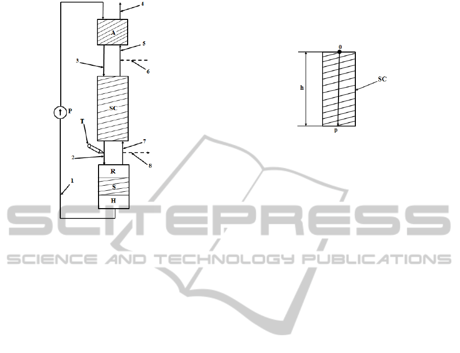
Figure 1: The separation plant.
regime, some connecting pipes are used to connect
pipes 6 and 8.In Figure 1, the hachured zones signify
that the corresponding elements present steel pack of
Helipack type. The steel pack has a determinant
contribution in the plant working, making possible
the
13
C isotope separation (Axente et. all, 1994).
The problem of
13
C separation is treated in a few
papers from the technical literature, for example in
(Li et. all, 2010), but the proposed solutions for
improving the separation process are not based on
using an advanced control strategy. Also, all the
control solutions are referring only to the
13
C isotope
concentration control at the base of SC (associated
to the position of T from Figure 1). At this moment,
the treated separation plant is controlled using an
on-off concentration controller which does not
ensure the necessary control accuracy and it
introduces undesired fluctuations in the system.
2 PROCESS MODELING
The
13
C isotope separation process is a distributed
parameter process (Li and Qi, 2011), the output
signal y (the
13
C concentration) depending both on
the independent variable time (t) and on the position
in the SC in relation to its height. The concentration
variation in relation to the position in the transversal
section of SC is insignificant and it is not considered
in the process model. In order to highlight the
second independent variable “length” notated with p,
the 0p axis from Figure 2 is defined. The origin 0 of
the 0p axis is the centre of the transversal section of
the SC from its upper part (the term transversal
section is referring to a section on which the height
direction (for example the 0p axis) is a vertical line).
Figure 2: The 0p axis.
Due to the fact that SC has a cylindrical form,
each transversal section is a circle. The diameter of
the transversal section is d = 2.5cm and the column
height is h = 300cm (Axente et. all, 1994).
Considering the previous aspects, the p independent
variable has the definition domain p
{[p
0
, p
f
] = [0,
h]}. The y(t,p) signal has an increasing evolution in
relation to the both independent variables, implying
that the approximating analytical solution which
describes the process work in transitory regime
contains two functional terms that have to be
determined, one in relation to t (F
t
(t)) and the second
one in relation to p (F
p
(p)). The modelling procedure
is valid for all working regimes, but only after the
CO
2
enters the first time in the SC through the pipe
8. First, the expression of the F
t
(t) function is
determined. The height equivalent to a theoretical
plate (HETP) is a function depending on the input
ethanolamine flow. Knowing that the dependence
between HETP and ethanolamine input flow F
in
is a
linear one (Axente et. all, 1994), the following
relation can be written:
HETP(t) = HETP
0
+ K
H
·(F
in
(t) – F
in0
), (1)
where HETP(t) is the instantaneous value of the
height of the equivalent plate, HETP
0
is the steady
state value of the height of the equivalent plate for
the ethanolamine input flow F
in0
= ct., K
H
is a
proportionality constant which makes the connection
between the ethanolamine input flow and HETP and
F
in
(t) is the instantaneous value of the ethanolamine
input flow. The proportionality constant K
H
is
determined using some experimental data resulted
from the plant. Each experiment is made measuring
the evolution in time of the output signal y(t,p) for
different step type variations of the input signal
F
in
(t). The value of the reference input flow is
chosen from the experimental data F
in0
= 367ml/h,
its corresponding HETP
0
having the value 4.64cm.
In (Axente et. all, 1994) it was proved that K
H
is
the gradient of the ramp resulted after the graphical
NeuralModelingandControlofa13CIsotopeSeparationProcess
255

representation of the function HETP
st
(F
in
), where
HETP
st
represents the steady state values of HETP
corresponding to different F
in
step signals.
Determining, also experimentally, that for F
in1
=
=460ml, HETP
st1
= 5.43, K
H
can be computed using
the relation:
in0in1
0st1
H
F -F
HETP - HETP
K 
,
(2)
resulting after computation K
H
= 0.0085(cm·h)/ml.
The instantaneous value of the number of the
theoretical plates is given by:
n(t) = h/HETP(t). (3)
Also, the isotope separation can be computed
using relation (4):
S(t) = α
n(t)
, (4)
where α = 1.01 is the elementary separation factor of
the
13
C isotope for the carbamate – CO
2
chemical
exchange procedure. Considering (1), the positive
value obtained for K
H
constant implies the increase
of HETP(t) at the increase of F
in
(t). Also, from (3)
and (4) the decrease of the number of theoretical
plates, respectively of the isotope separation value,
results. The main consequence of the last two
remarks is the fact that the y(t,p) signal decreases at
the F
in
(t) increasing, respectively the y(t,p) signal
increases at the F
in
(t) decreasing. From the physical
point of view, this phenomenon is explained due to
the fact that lower the value of the input
ethanolamine flow F
in
(t) is, the longer the contact
duration between the carbamate and CO
2
in SC is,
the chemical exchange between the two chemical
elements being a more efficient one.
Also, the isotope separation is given by the
relation:
0
inff
y
)(t)F)(p,y(t
S(t) 
,
(5)
where y
0
= 1.108% represents the natural abundance
of the
13
C isotope and y(t
f
,p
f
)(t) is the steady state
value of the output signal for a certain input step
type signal which would have the instantaneous
value of the signal F
in
(t), considering that
p = p
f
=300cm. From (4) and (5), it results that:
n(t)
0inff
αy)(t)F)(p,y(t 
,
(6)
or
)t(Sy)(t)F)(p,y(t
0inff


.
(7)
The
13
C concentration increase over the initial
value y
0
, in steady state regime, is given by:
)1)t(S(y
)1α(yy)(t)F)(p,y(t
0
n(t)
00inff


.
(8)
The final input signal in the process is defined
by:
)1)t(S(y(t)u
0f



.
(9)
Obviously, if F
in
(t) is a step type signal it results
that the u
f
(t) signal is a step type signal, too.
The isotope separation process is a first order
one, being characterized by only one time constant.
The time constant of the process is experimentally
determined and if the experiment based on a step
type variation of the input signal F
in
(t) is made for
p = p
f
, it can be determined using the tangent
method, resulting the value T
pf
= 14h. If the same
experiment is repeated, but the measurement of the
output signal y(t,p) is made in the close
neighbourhood of the origin 0 on the 0p axis (for the
value p = 0
+
), after applying the tangent method, it
results for the process time constant the value
T
p0
= 2h.
From these experimental identifications of the
two time constants, it results that the process time
constant increases progressively from the upper part
to the lower part of SC along the 0p axis. Next, in
this paper, a linear increasing evolution of the T time
constant of the process along the 0p axis is
considered, given by the relation:
f
p0pfp0
p
p
)TT(TT 
,
(10)
where p
f
= h. From (10) it can be remarked that
T = T(p), but the changing of the value of the p
independent variable is not made continuously. The
p value changing is made at discrete time moments
through the changing of the transducer T position
inside the SC along the 0p axis. The commutations
of the p independent variable can be viewed as step
type signals.
The first order differential equation which
describes the relation between the final input signal
u
f
(t) and the function F
t
(t) (F
t
(t) being the solution of
this equation) is:
)t(u
T(p)
1
)t(F
T(p)
1
dt
)t(dF
ft
t
 .
(11)
In the previous equation, the p independent
variable change implies the value changing of the
process time constant T(p), the effect of such a
variation influencing the F
t
(t) function only in
transitory regime. Consequently, F
t
depends on both
independent variable F
t
(t,p) only in the commutation
moments of the p independent variable and only
ICINCO2015-12thInternationalConferenceonInformaticsinControl,AutomationandRobotics
256

when this commutation takes place in transitory
regime. Also, the F
t
(t) function represents the
13
C
concentration evolution in time over the value y
0
until the value y(t
f
,p
f
) for a certain value of F
in
(t). If
the value of the p variable is changed, the speed
evolution of the F
t
(t) function is adapted, but its
steady state value remains at y(t
f
,p
f
). This problem is
solved introducing in the approximating analytical
solution the F
p
(p) function.
The F
p
(p) function can be determined in two
stages. Firstly, the F
p1
(p) function is determined. The
y(t,p) evolution in relation to the p independent
variable for t = t
f
and for a certain constant value of
the F
in
signal is given by the relation:
)n(t
0f
f
α · y = p),y(t ,
(12)
As it results from (12), the evolution in time of
the y(t
f
,p
f
) signal has a hyperbolic form. Using a
mathematical procedure based on an interpolation
method, the y(t
f
,p) signal can be approximated by a
F
p1
(p) function of the form:
)F)t(F(K430
p
0p1
in0inP
e1)-α(y = (p)F


,
(13)
where C = 430cm is a SC constant determined
through interpolation and K
P
= 0.7527(cm·h)/ml
results using two consecutive determined sets of
values {F
in
, P}. The “length” constant P is:
P = 430 + K
P
·(F
in
(t) – F
in0
). (14)
As it can be remarked, the F
p1
(p) function can be
modelled using only one “length” constant P. Also,
from (14), it results that P is a function of the input
ethanolamine flow P(F
in
(t)), implicitly a function of
time P(t). It results that F
p1
is a function depending
on F
in
(t) (F
p1
(F
in
(t),p) and implicitly on both
independent variables t and p (F
p1
(t,p)).
Secondly, the function F
p2
= F
p1
(F
in
(t),p
f
) is
determined. The final form of the F
p
(p) function
results using the relation:
0finp1
0inp1
0p2
0inp1
inp
y-)p(t),(FF
y-p)(t),(FF
y-F
y-p)(t),(FF
= (t))F(p,F


,
(15)
this function depending on the input flow F
in
(t), too.
Also, the final form of the approximating
analytical solution is given by:
y
AN
(t,p) = y
0
+ F
t
(t)·F
p
(p,F
i
n
(t)) . (16)
Due to the facts that, F
p
= F
p
(F
in
(t),p), it results as
ratio between two other functions ((F
p1
– y
0
) and
(F
p2
– y
0
)) and for some particular cases F
t
= F
t
(t,p),
getting to the conclusion that the treated separation
process is a strong non-linear one.
3 LEARNING THE PROCESS
BEHAVIOUR USING NEURAL
NETWORKS
The approximating analytical solution from (16)
which describes the working of the separation
process, the process being a distributed parameter
one (Smyshlyaev and Krstic, 2005), has a very
complex structure. Considering this aspect, the
analytical solution is decomposed in some more
simple mathematical components. Each resulted
mathematical component is modelled using a neural
network and, after that, in order to obtain the model
of the entire analytical solution, the resulted neural
networks are properly interconnected between them.
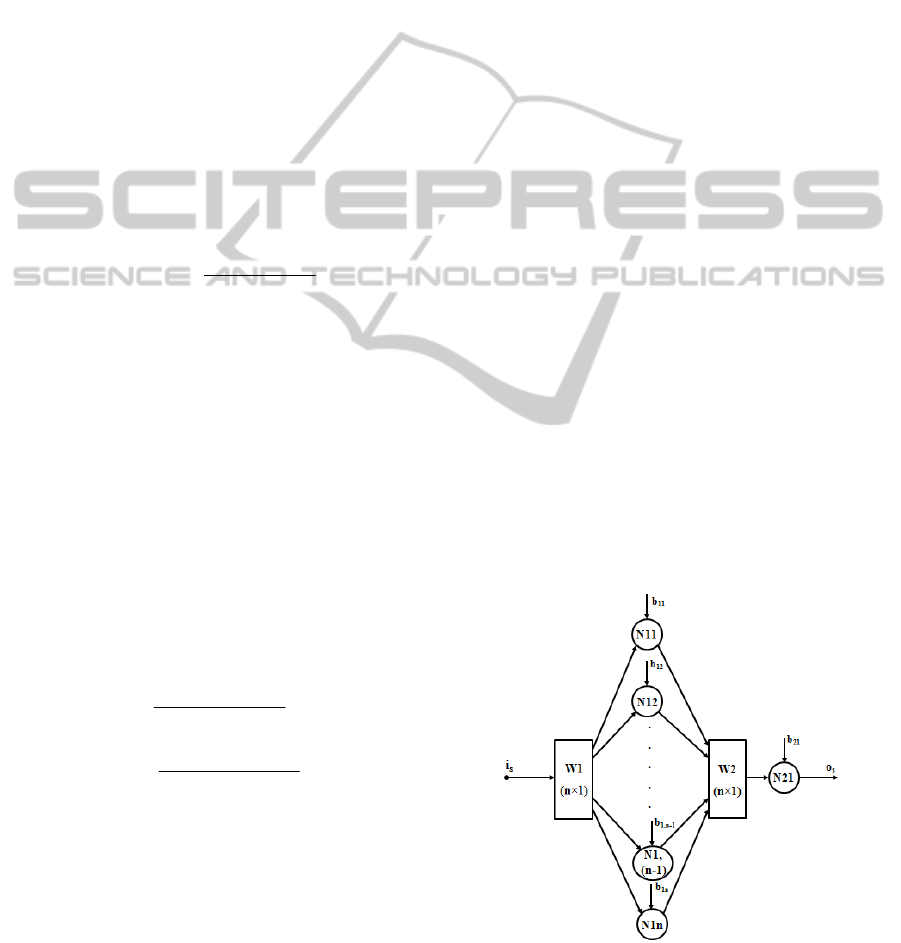
The two types of neural structures used to learn
(Borges, 2011) the behaviour of the components of
the analytical solution are the forward fully
connected neural networks and the autoregressive
fully connected networks with exogenous inputs
(Haykin, 2009). The two types of neural networks
are presented schematically in Figures 3 and 4. In
both cases, i
s
represents the input signal in the neural
network and o
s
represents the output signal from the
neural network. In all the cases from this paper, the
network from Figure 3 contains non-linear neurons
in the hidden layer (N
1i
neurons, where i = 1,…,n)
having hyperbolic tangent activation functions).
Also, in all the cases, the N21 neuron is linear
(having linear activation function (Maren et. all,
1990; Norgaard et. all, 2000)).
Figure 3: The forward fully connected network.
NeuralModelingandControlofa13CIsotopeSeparationProcess
257

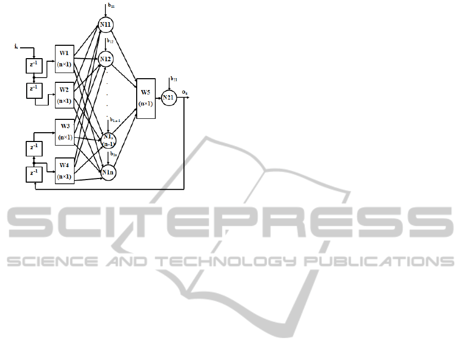
Figure 4: The autoregressive fully connected network with
exogenous inputs.
The W1 and W2 vectors are column vectors
containing the weights that make the connection
between the input layer and the hidden layer,
respectively between the hidden layer and the output
layer. The n dimension (the dimension of the hidden
layer) can be singularized for each application in
part. The output signal o
s
, for the general structure
from Figure 3 is given by the relation:
o
s
= [tanh(i
s
·W1
T
+ B1
T
]·W2 + b21, (17)
where B1 is a column vector containing the bias
values of the neurons from the hidden layer, b21 is
the bias value of the N21 neuron, the superscript
T
signifies that the corresponding vector is considered
in transposed form and the notation “tanh” signifies
the application of the hyperbolic tangent functions to
all the elements of the corresponding vector.
The structure from Figure 4 is used in the case
when the work of the components is expressed using
differential equations. The elements z
–1
represent
delay lines used both on the input and on the
feedback signal, in order to memorize the previous
values of the two signals. The connection between
the input layer (formed by the input signal and the
feedback signal) and the hidden layer is made
through the column vectors W1 and W2,
respectively W3 and W4, all of them containing
weights. W5 has the same significance as W2 in the
case of Figure 3 and the dimension n is singularized,
also, for each application in part. In the case of the
network from Figure 4, all the neurons are linear.
The o
s
signal is given by the relation:
o
s
(k) = [W1
T
·i
s
(k–1)+ W2
T
·i
s
(k–2)+ W3
T
·
·o
s
(k–2)+ W4
T
·o
s
(k–1)+ B1
T
]·W5 + b21,
(18)
where B1, b21 and
T have the same significance as
in the case of relation (17), respectively the sequence
(k) represents the current value of the signals, and
the sequences (k–1) and (k–2) represent the previous
two values of the signals. If only one unit line is
necessary for a certain application both on the input
and on the feedback signals, the same presented
structure can be used considering the elements of the
matrices W2 and W3 equal to 0 (Vălean, 1996).
The implementation of the approximating
analytical solution from (16) using neural networks
is presented in Figure 5. The neural networks noted
with NN are trained in order to learn the functional
dependence between the corresponding input and
output signals. Practically, the neural structure from
Figure 5 resulted following the relations (1)-(16) and
interconnecting the component neural networks,
obviously processing mathematically the signals that
occur in the structure. All the neural networks from
Figure 5, instead of NN4 are forward fully
connected ones with n = 10. They are trained using
1000 input-output data pairs and considering, also, a
ramp type variation of the corresponding input
signals. In all cases, as training algorithm, the
Levenberg-Marquardt back-propagation algorithm is
used. The maximum number of training epochs was
fixed to 20000, obtaining in all cases very small
error values (values proportional with 10
-13
; the
quality indicator is considered the mean square
error). The neural network NN4 implements the
integration function.
In this case the autoregressive fully connected
network with exogenous inputs structure from
Figure 4 is used, considering all the elements of the
vectors W2 and W3 equal to 0 (only 1 unit delay
both on the input and on the output signals). Also, in
this case n = 7. The same number of input-output
data pairs and the same training algorithm are
considered as in the case of the other Neural
Networks from Figure 5, but a white noise variation
of the input signal. The imposed value of the mean
square error is reached after 15 training epochs. The
neural model implemented in Figure 5 and
associated to the analytical solution from (16) will
be used as the process Reference Model in the IMC
control structure.
4 THE PROPOSED CONTROL
STRUCTURE
The control structure based on the Internal Model
Control (IMC) strategy (Love, 2007; Golnaraghi et.
ICINCO2015-12thInternationalConferenceonInformaticsinControl,AutomationandRobotics
258

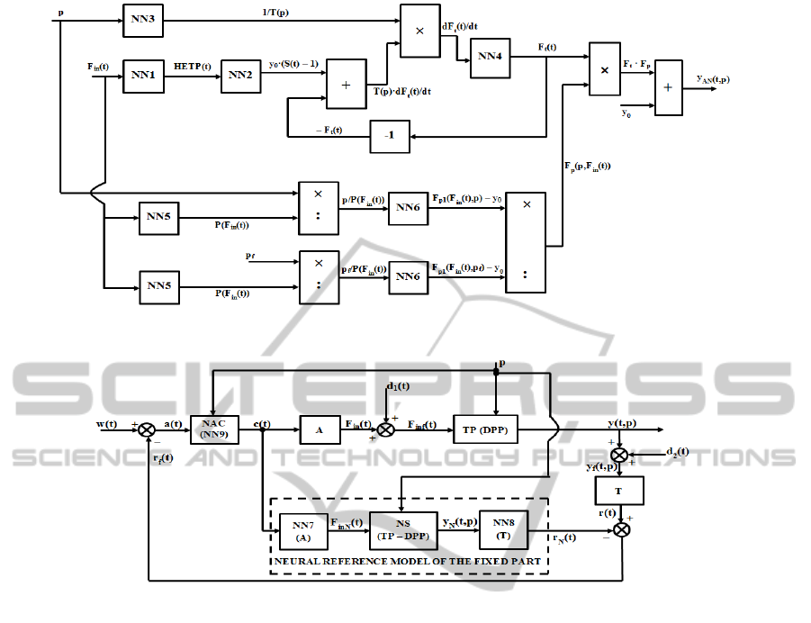
Figure 5: The implementation of the approximating analytical solution using neural networks.
Figure 6: The proposed IMC structure.
all, 2009), proposed to be used for the concentration
control of the
13
C isotope, is presented in Figure 6.
The elements from the direct physical channel of
the structure are: the actuator A (the pump P from
Figure 1), the distributed parameter (DPP)
technological process (TP) and the transducer T (the
same transducer as in Figure 1). Also, the elements
from the direct reference channel represent the
neural networks that describe the work of the
elements from the physical direct channel: NN7 for
A, NS (neural structure from Figure 5) for the TP
(DPP) and NN8 for T. The three neural models
connected in series represent the Neural Reference
Model of the Fixed Part of the system. Also the
element NAC is the Neural Adaptive Controller
modelled using the neural structure NN9. From the
mathematical point of view, the NAC controller is a
distributed parameter controller. The term
“distributed parameter controller” is referring to the
fact that one of the controller parameters (the main
parameter) depends on the value of the p
independent variable. This term does not have the
meaning of a spatial distribution of the generated
control signal. Also the significance of the notations
regarding the signals from Figure 6 is: w(t) –
reference signal, c(t) – control signal, F
in
(t) –
– actuating signal (the input flow of ethanolamine),
d
1
(t) – disturbance signal which affects directly the
actuating signal, F
inf
(t) – disturbed actuating signal
(the final value of the ethanolamine input flow),
y(t,p) – output signal (the
13
C isotope concentration),
d
2
(t) – disturbance signal which affects directly the
output signal, y
f
(t,p) – disturbed output signal due to
the effect of d
2
(t), respectively r(t) – feedback signal.
Also, the F
inN
(t), y
N
(t,p), and r
N
(t) signals have
the same significance as the signals F
in
(t), y(t,p) and
r(t), but represent output signals from the
corresponding elements of the Reference Model of
the Fixed Part. These signals are not disturbed, the
disturbances not affecting the reference direct
channel of the system. The final feedback signal
r
f
(t) = r(t) – r
N
(t) represents a measure of all
disturbances effects that affect in a negative manner
the work of the physical direct channel (d
1
(t), d
2
(t),
but also the parametric disturbances (variations in
time of the parameters of the elements A, TP and
T)). Also a(t) = w(t) – r
f
(t) is the error signal. It can
be remarked that the value of the p independent
NeuralModelingandControlofa13CIsotopeSeparationProcess
259

variable is transmitted to both direct channels and to
the controller.
The structure from Figure 6 can work, in the case
the p variable value is not transmitted to the
reference direct channel, but this case is not treated
in this paper. Also, the structure can be adapted for
the case when the automatic determination of the p
value is necessary (Muresan and Abrudean, 2010),
case which also, is not treated in this paper. The
work of the actuator A, it having a linear behaviour,
is expressed using a second order transfer function.
The values of the time constants of the actuator are:
T
A
= 0.1min (the time constant of the actuator) and
T
1
= 2min (the time constant introduced using an
electronic equipment in order to “delay” the
propagation of the control signal to the actuator).
Also, the proportionality constant of the actuator
K
A
= -56.25 ml/(h·mA). The generated output signal
represents the value of the ethanolamine flow which
has to be subtracted from F
inmax
in order to obtain the
F
in
signal. This adjustment is necessary due to the
fact that the plant technological start is made using
F
inmax
. The A element is modelled using the neural
network 7 (NN7). NN7 has exactly the structure
from Figure 4, for n = 10. Also all the delay lines
from Figure 4 are necessary due to the fact that the
actuator model is of second order. The network NN7
is trained using the same training algorithm as in the
case of NN4, the same type of input signal and 500
pairs of input-output data. The imposed mean square
error of is reached after 17 training epochs. The used
sampling time, in this case, has the value
T
s
= 0.036 min. This value is much smaller than the
value of the sampling time used for the training of
all neural networks from the previous Paragraph (3)
(T
s
= 30 min) due to the much smaller time constants
values of the actuator comparing to the value of the
time constant of the technological process.
The transducer T model is expressed using a first
order transfer function with K
T
= 5.7143mA/% (the
proportionality constant of the transducer) and
T
T
= 6min (the time constant of the transducer). The
computation of K
A
and K
T
proportionality constants
is made taking in consideration the fact that the
automation equipment used for this application
works with unified current signals. This model is
learned using the NN8 neural network from
Figure 6. The network parameters and the training
parameters are the same as in the case of the NN4
training, with the exception that T
s
= 0.09min.
The controller is tuned in order to compensate
the main time constant of the process T(T(p)). The
mathematical model which describes the controller
work in time domain is expressed using the
following differential equation:
a(t)
d
t
da(t)
T(p)c(t)
d
t
dc(t)
T
f
 ,
(19)
where T
f
is the time constant of the first order filter
used in order to obtain the controller feasibility
(T
f
< T(p)). The control signal c(t) represents the
solution of the equation (19). At the changing of the
p independent variable value, the value of the
process time constant is modified and from (19) it
results that the value of the T(p) time constant of the
controller is modified, too, in order to be adapted to
the new time constant of the process. This
explanation implies the term “adaptive controller”.
Also the modification of the T(p) value is made
through the value of p independent variable, being
justified the abstract term of “distributed parameter
controller”. The implementation of the controller
using three neural networks interconnected between
them using mathematical operators, is presented in
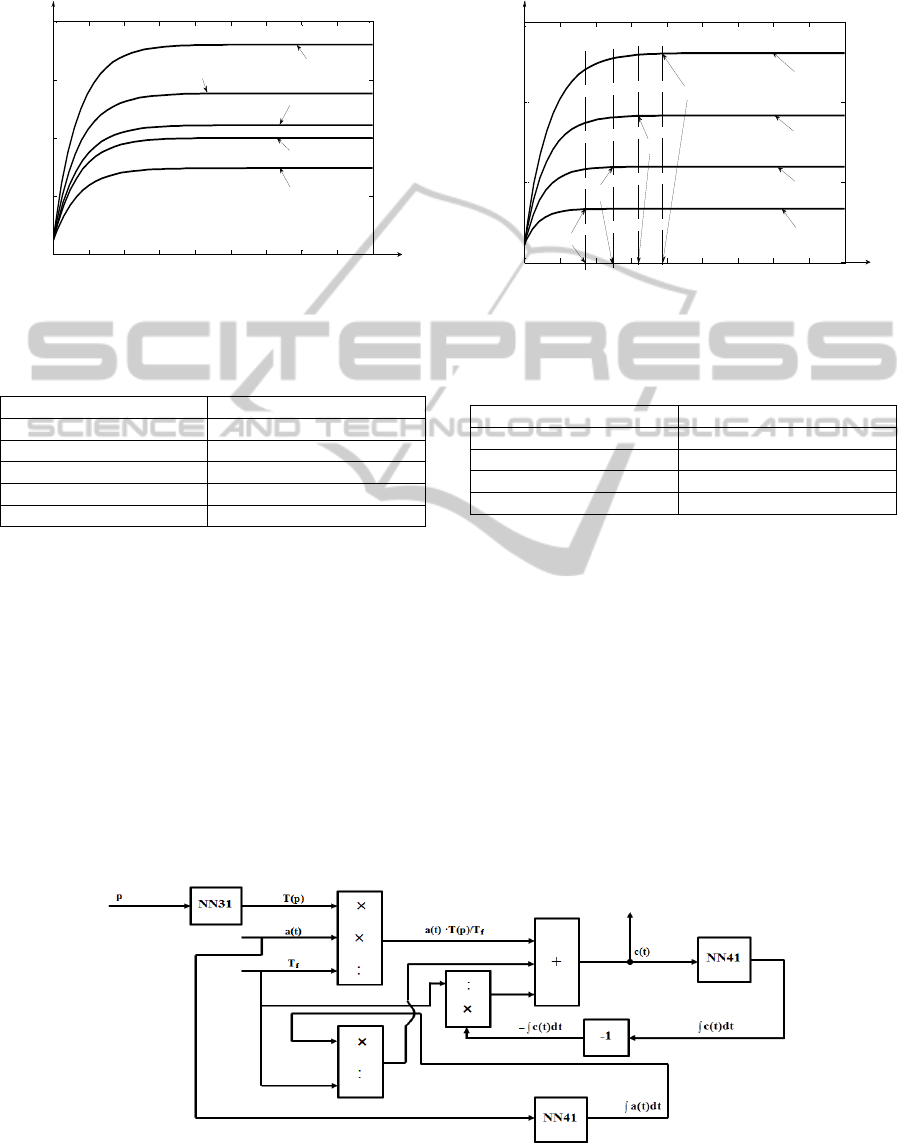
Figure 7. The NN31 has the same structure as NN3
from Figure 5, generating at the output the value
T(p). Also, the NN41structures have the same
structure as NN4 from Figure 5, implementing the
integration operation. The training procedures and
parameters for the two types of neural networks
from Figure 7 are the same as in the case of NN3
and NN4 from Figure 5, with the exception of the
sampling time (in this case T
s
= 3min). In the case
when the
13
C isotope concentration control is made
in the point p = p
f
, the value T
f
= 8h represents a
good compromise between the system stability and
the structure performances. Also, for this value, the
usage of the control signal is feasible from its
saturation values avoidance point of view.
Having the neural models of the elements A, TP
and T, practically the model of the Reference Model
of the Fixed Part can be implemented, for example,
on a process computer and the structure from
Figure 6 can be used. The model of the controller,
also expressed using a neural networks structure, can
be implemented on a computation equipment, too.
5 SIMULATION RESULTS
The simulations (Colosi et. all, 2013) are made in
MATLAB/Simulink. First the validity of the
analytical solution from (16) is verified. In Figure 8
is presented the comparative graph between 5 step
responses of the separation column model expressed
through the mentioned analytical solution, if the
simulation is made for p = p
f
. The values of the
considered input step type variations are F
in
 {200;
ICINCO2015-12thInternationalConferenceonInformaticsinControl,AutomationandRobotics
260

280; 367; 416; 600}ml/h. The steady state values of
the
13
C concentration isotope (y(t
f
,p
f
)) are
centralized in Table 1.
0 20 40 60 80 100 120 140 160 180
1
1.5
2
2.5
3
TIME [h]
y(t,p) [% ]
Fin = 280ml/h
Fin = 367ml/h
Fin = 416ml/h
Fin = 600ml/h
Fin = 200ml/h
Figure 8: Open loop responses of the determined process
model for different values of the input signal.
Table 1: The simulation results associated to Figure 8.
F
in
[ml/h] y(t
f
,p
f
) [%]
200 2.8
280 2.3818
367 2.1083
416 2
600 1.7392
Comparing to the experimental data from
(Axente et. all, 1994), it results that the determined
approximating analytical solution describes the
process work with high accuracy, the differences
occurring only at the third decimal. Also, in Table 1
and Figure 8 the increasing evolution of the
13
C
isotope concentration at the decrease of the value of
the input ethanolamine flow is highlighted.
In Figure 9 is presented the comparative graph
between 4 step responses of the separation column
model expressed through the mentioned analytical
solution, if the input flow of ethanolamine presents a
step type variation with the value F
in
= 300ml/h, for
different values of the p independent variable
p

{p
f
/4; p
f
/2; p
f
/4·3; p
f
}[cm]. The steady state
values of the
13
C isotope concentration (y(t
f
,p)) from
Figure 9 are centralized in Table 2.
0 20 40 60 80 100 120 140 160 180
1
1.5
2
2.5
TIME [h]
y(t,p) [% ]
ts1
ts2
ts3
ts4
p = pf
p = pf/4*3
p = pf/4
p = pf/2
Figure 9: Open loop responses of the determined process
model for different values of the p independent variable.
Table 2: The simulation results associated to Figure 9.
p [cm] y(t
f
,p) [%]
p
f
/4 1.3345
p
f
/2 1.5971
p
f
/4·3 1.917
p
f
2.3069
From Figure 9 and Table 2, the decreasing
evolution of the process response in relation to the
decrease of the p independent variable is
highlighted. From the mathematical point of view,
this aspect is explained due to the increasing
evolution of the F
p
function in relation to the
increase of p. From the physical point of view, this
aspect is explained due to the increase evolution of
the number of the theoretical plates in relation to the
increase of p. Also, from Figure 9 it can be remarked
that lower the value of p is, lower the value of the
process settling time is (t
s1
< t
s2
< t
s3
< t
s4
). This
phenomenon is explained due to the decreasing
evolution of the T(p) process time constant at the
decrease of p.
Figure 7: The implementation of the controller using neural networks.
NeuralModelingandControlofa13CIsotopeSeparationProcess
261

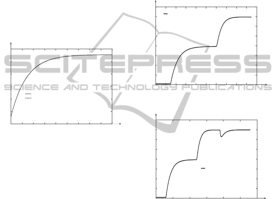
In Figure 10, the comparative graph between the
process response (modelled through the analytical
solution) and the process response (modelled
through the neural structure implemented in Figure
5) is presented. Practically, the differences between
the two curves from Figure 10 cannot be
distinguished, resulting the high validity of the
Neural Reference Model of the Fixed Part of the
control system from Figure 6 (the NS element from
the Reference Model has the main weight in it). The
square mean error between the two curves from
Figure 10, computed for 453 pairs of values
associated to the two responses, has the value
E
mp
= 0.0023%, considered insignificant for this
application.
0 10 20 30 40 50 60 70 80 90
1
1.2
1.4
1.6
1.8
2
2.2
TIME [h]
y(t,p) [% ]
Output generated by the analytical solution
Output generated by the neural network
Figure 10: The validation of the neural model associated
to the technological process.
In Figure 11, the response of the control system
from Figure 6 is presented. Firstly, between the time
moments t
1
= 30h and t
2
= 120h, the plant works in
starting regime, the ethanolamine flow being
maintained at F
inmax
. After the
13
C isotope
concentration (the output signal) gets steady to the
value 1.492%, the structure can be used to assure a
certain value of the y(t,p) signal. The simulation
from Figure 11 is made for p = p
f
. After the moment
t
2
, the concentration reference is set to the value
1.795%. From the Figure it can be remarked that this
value is reached after approximately 40h, much
faster than in open loop regime (case of t
s4
from
Figure 9 which has the value approximately equal to
78h). Also it can be remarked that the steady state
error a
st
= 0% and the overshoot %0σ  (a very
important constrain imposed to the treated type of
system).
In Figure 12, the simulation from the Figure 11 is
repeated until the time moment t
3
= 190h. In this
moment the disturbance d
2
(t) of step type with the
value –0.1% occurs in the system. From Figure 12, it
results that the effect of the disturbance is efficiently
rejected by the controller after 50h the concentration
value being brought back to the value imposed
through the reference signal.In both the cases of the
simulations from Figures 11 and 12, the saturation
limits of the control respectively of the actuating
signals (both the minimum and maximum limits) are
not reached, the usage of the controller being
feasible.
0 20 40 60 80 100 120 140 160 180 200
1.1
1.2
1.3
1.4
1.5
1.6
1.7
1.8
1.9
TIME [h]
y(t,p) [% ]
Automatic control system response
Figure 11: The automatic control system response.
0 50 100 150 200 250 300
1.1
1.2
1.3
1.4
1.5
1.6
1.7
1.8
1.9
TIME [h]
y(t,p) [% ]
The automatic control system response
Figure 12: The automatic control system response, for the
case when a disturbance signal occurs in the system.
6 CONCLUSIONS
An original solution for the mathematical modelling
of a separation technological is presented in this
paper. Also, a solution for the automatic control of
the
13
C isotope concentration is presented based on
the IMC strategy.
In order to implement the Reference Model of
the system Fixed Part, the neural networks are used.
ICINCO2015-12thInternationalConferenceonInformaticsinControl,AutomationandRobotics
262

These elements are original ones, too, due to the fact
that a distributed parameter technological process is
included in an IMC control structure and the model
of this type of process is learned using neural
networks. The work of A and T elements (Figure 6)
is learned using neural networks in order to preserve
the unitary character of the solution and the high
accuracy of the Fixed Part mathematical model.
The neural networks are used, also, for
implementing the adaptive controller, respectively
the term “distributed parameter controller” is
introduced and defined.
The process model validity and the high
performances of the proposed control structure are
proved through the simulations from Paragraph 5.
The control structure is tested in the case when a
disturbance signal occurs in the system. As it can be
remarked from Figure 12, the effect of the
disturbance is rejected with high efficiency.
ACKNOWLEDGEMENTS
The research activity that helped the authors to
elaborate the paper is supported through the research
projects no. 30141/12.12.2014 and no. 30104/2014,
financed by the Technical University of Cluj-
Napoca.
REFERENCES
Axente, D., Abrudean, M., Bâldea, A., 1994.
15
N,
18
O,
10
B,
13
C Isotopes Separation trough Isotopic
Exchange, Science Book House.
Borges, R. V., 2011. Learning and Representing Temporal
Knowledge in Recurrent Networks. In IEEE
Transactions on Neural Networks, Vol. 22, Issue 12,
pp. 2409 – 2421.
Coloşi, T., Abrudean, M., Ungureşan, M.-L., Mureşan, V.,
2013. Numerical Simulation of Distributed Parameter
Processes, Springer.
Dang, H., Rochelle, G. T., 2003. CO2 absorption rate and
solubility in monoethanolamine/ piperazine/ water. In
Separation Sci. & Tech., Vol. 38 (2), pp. 337–357.
Dugas, R., Rochelle, G., 2009. Absorption and desorption
rates of carbon dioxide with monoethanolamine and
piperazine. In Energy Procedia, Vol. 1 (1), pp. 1163–
1169.
Golnaraghi, F., Kuo, B. C., 2009. Automatic Control
Systems, 9
th
edition, Wiley Publishing House.
Haykin, S., 2009. Neural Networks and Learning
Machines, Third Edition, Pearson Int. Edition.
Li, H.-L., Ju, Y.-L., Li, L.-J., Xu D.-G., 2010. Separation
of isotope
13
C using high-performance structured
packing. In Chemical Engineering and Processing:
Process Intensification, Vol. 49 (3), pp. 255–261.
Li, H.-X., Qi, C., 2011. Spatio-Temporal Modeling of
Nonlinear Distributed Parameter Systems: A
Time/Space Separation Based Approach, 1st Edition,
Springer.
Love, J., 2007. Process Automation Handbook, 1 edition,
Springer.
Maren, A., Harston, C., Pap, R., 1990. Handbook of
Neural Computing Applications, Academic Press.
Mureşan, V., Abrudean, M., 2010. Temperature Modelling
and Simulation in the Furnace with Rotary Hearth. In
Proc. of IEEE AQTR–17
th
ed., Cluj-Napoca,
Romania, pp. 147-152.
Norgaard, M., Ravn, O., Poulsen, N.K., Hansen, L.K.,
2000. Neural Networks for Modelling and Control of
Dynamics Systems, Springer.
Smyshlyaev, A., Krstic, M., 2005. Control design for
PDEs with space-dependent diffusivity and time-
dependent reactivity. In Automatica, Vol. 41, pp.
1601-1608.
Vălean H., 1996. Neural Network for System
Identification and Modelling. In Proc. of Automatic
Control and Testing Conference, Cluj-Napoca,
Romania, 23-24 May, pp. 263-268.
NeuralModelingandControlofa13CIsotopeSeparationProcess
263