Linear Software Models: Equivalence of Modularity Matrix to Its

Modularity Lattice

Iaakov Exman

and Daniel Speicher

Software Engineering Dept., The Jerusalem College of Engineering – JCE-Azrieli, Jerusalem, Israel

Bonn-Aachen International Center for Information Technology, University of Bonn, Bonn, Germany

Keywords: Linear Software Models, Modularity Matrix, Modularity Lattice, Formal Concept Analysis, Equivalence.

Abstract: Modularity is an important feature to solve the composition problem of software systems from subsystems.

Recently it has been shown that Software systems’ Modularity Matrices linking structors to functionals can

be put in almost block-diagonal form, where blocks reveal higher-level software modules. An alternative

formalization has been independently proposed using Conceptual Lattices linking attributes to objects. But,

are these independent formalizations related? This paper shows the equivalence of Modularity Matrices to

their respective Modularity Lattices. Both formalizations support the simplest form of software

composition, i.e. linear composition, expressed as an addition of independent components. This equivalence

has both theoretical and practical advantages. These are illustrated by comparison of both representations

for a series of case studies.

1 INTRODUCTION

Composition of software systems from subsystems

and basic components is an important problem. It is

widely accepted that modularity is essential to solve

this problem. Two independent approaches have

formalized modularity for the software composition

problem, relying on algebraic structures.

One approach uses Modularity Matrices linking

structures to their functionality. Another approach

represents relations between objects and attributes as

Lattices of formal concepts. This work shows the

equivalence of the matrix and lattice approaches,

assuring that results in either approach are valid in

the other approach as well. In other words, they are

alternative representations of the software system.

1.1 Modularity Matrix Concepts

A Modularity Matrix displays relations between two

kinds of architectural entities in a software system:

structors, the columns, and functionals, the rows.

Structors generalize UML classes (i.e. a class,

interface, aspect, sets of related classes, such as

design patterns). Functionals generalize class

functions (i.e. a method, families of functions, such

as trigonometric functions). Each 1-valued matrix

element links a structor to a provided functional.

Functionals are potential functions, not necessarily

invoked in the system. In (Exman, 2012) it was

shown by linear algebra arguments that:

• A Modularity Matrix is square – if its structors

are linearly independent and also its functionals

are linearly independent;

• A Modularity Matrix is block-diagonal – if

certain structor sub-sets provide sub-sets of

functionals, disjoint to other sub-sets; each block

is an independent module.

In a standard Modularity Matrix all the matrix

elements outside modules are zero-valued. A block-

diagonal matrix is got by reordering rows/columns.

Modularity Matrix elements are numbers used in

actual calculations. For instance, to compare the

relative modularity of different software designs of a

system one calculates the Matrix M diagonality, with

elements M

(row j, column k) and dimension N:

() () ()

iagonality M Trace M offdiag M=−

(1)

where

() *| |

offdiag M M j k

=−



(2)

1.2 Modularity Lattice Concepts

A conceptual lattice displays relations between two

109

Exman I. and Speicher D..

Linear Software Models: Equivalence of Modularity Matrix to Its Modularity Lattice.

DOI: 10.5220/0005557701090116

In Proceedings of the 10th International Conference on Software Paradigm Trends (ICSOFT-PT-2015), pages 109-116

ISBN: 978-989-758-115-1

 2015 SCITEPRESS (Science and Technology Publications, Lda.)

kinds of entities: attributes and objects. Attributes

express the concepts’ intent, and object sets express

the concepts’ extent. The Top lattice node has empty

set intent and an extent as the set of all objects.

Mutatis mutandis the Bottom lattice node has empty

set extent and an intent as the set of all attributes.

A conceptual lattice is built by first preparing its

formal context, i.e. a table displaying which objects

have certain attributes, marked by X signs. In

contrast to the Modularity Matrix, the formal context

has not been defined as a matrix with numerical

matrix elements, allowing calculations. Moreover,

there are no underlying linear algebra theorems on

the formal context, such as being square or block-

diagonal. A formal context may be a rectangular

table without any specific requirements.

In this work, we make the unique decision of

generating conceptual lattices directly from given

Modularity Matrices, with the expectation that the

resulting Modularity Lattices carry on the

characteristic properties of these matrices. This work

aims to show that this is indeed the case.

To show the equivalence of a modularity matrix

to a modularity lattice, we choose to match between

matrix ‘structors’ and the lattice intent (viz.

‘attributes’) on the one hand, and match between

matrix ‘functionals’ and lattice extent (viz. ‘objects’)

on the other hand. A link between a structor and a

functional corresponds either to an attribute in the

same node as its object, or to an attribute in a node

connected to a node by a downward set of edges in

the Lattice, not passing through Top or Bottom.

The conceptual justification for this matching is

clarified as follows. UML classes represent concepts

with definite intents. For instance, the class “car” is

a type of vehicle with the intent of travelling on

roads. Cars have wheels, their speed and travelled

distance may be calculated by suitable functions (the

extent). The class “airplane” is another type of

transportation medium with a different intent, viz. to

travel by flying. Airplanes also have wheels, their

speed is also calculated by suitable functions. Thus

different classes have clearly different intents, but

may have similar extents.

Software conceptual lattices are a broader

subject than implied by the above simple examples.

They deserve extensive discussion, which is outside

of this paper scope. Here we focus on the

equivalence of Modularity Matrices and Modularity

Lattices. For further details on formal concepts, see

(Ganter, 1999), (Ganter, 2005), (Belohlavek, 2008).

The remaining

of this paper is organized as

follows. Section 2 refers to related work. Section 3

displays an introductory example. Section 4

formulates theoretical considerations. Section 5

deals with heuristics for modules’ decoupling.

Section 6 presents canonical case studies. Section 7

shows a larger system case study. The paper is

concluded by a discussion in section

2 RELATED WORK

In this work we refer to the modularity matrix – e.g.

(Exman, 2014). Other matrices have also been used

in the context of modularity. For instance, the

Design Structure Matrix (DSM) proposed in

(Steward, 1981), and incorporated in ‘Design Rules’

(Baldwin, 2000). It has been applied in various

contexts – see e.g. (Cai, 2006).

Two essential differences between DSM and the

modularity matrix are: a- Linearity as an essential

idea of the modularity matrix; b- Both DSM

dimensions are labelled by the same structures.

The modularity matrix, in contrast to the DSM,

displays pairs of different entities, viz. structors to

functional links. The use of pairs of entities was

important to suggest the correspondence to

conceptual lattices, as the latter also refer to pairs of

entitities, viz. attributes and objects.

Conceptual lattices, generally known as part of

Formal Concept Analysis (FCA) were introduced in

(Wille, 1982). There are many available generic

overviews describing mathematical foundations

(Ganter, 1999), applications (Ganter, 2005) and

surveys of the field (Belohlavek, 2008).

FCA has been used as a technique for

modularization and system design. This includes

works such as (Lindig, 1997), (Siff, 1999) and

(Snelting, 2000). A specific usage of conceptual

lattices for software engineering is found in

(Heckmann, 2012).

3 INTRODUCTORY EXAMPLE:

COMMAND DESIGN PATTERN

The Command software design pattern, in the GoF

book (Gamma, 1995), serves as an introductory

example. The pattern decouples an object invoking

an action, say clicking a “Print” button, from another

object that actually prints a file. The pattern enables

generic features, such as Undo and Redo,

independently of the specific commands’ nature.

3.1 Command Modularity Matrix

The six structors in the Command Modularity Matrix

ICSOFT-PT2015-10thInternationalConferenceonSoftwareParadigmTrends

110

are in the list of Participants in the GoF book: an

abstract command (cmd), a concrete command (say,

Print File), an invoker (a button), a receiver (a file to

be printed), a client (initializes the application) and

history (enables undo). The Pattern functionals are:

execute, undo, create objects, bind command-to-

button, set-receiver, and the receiver action.

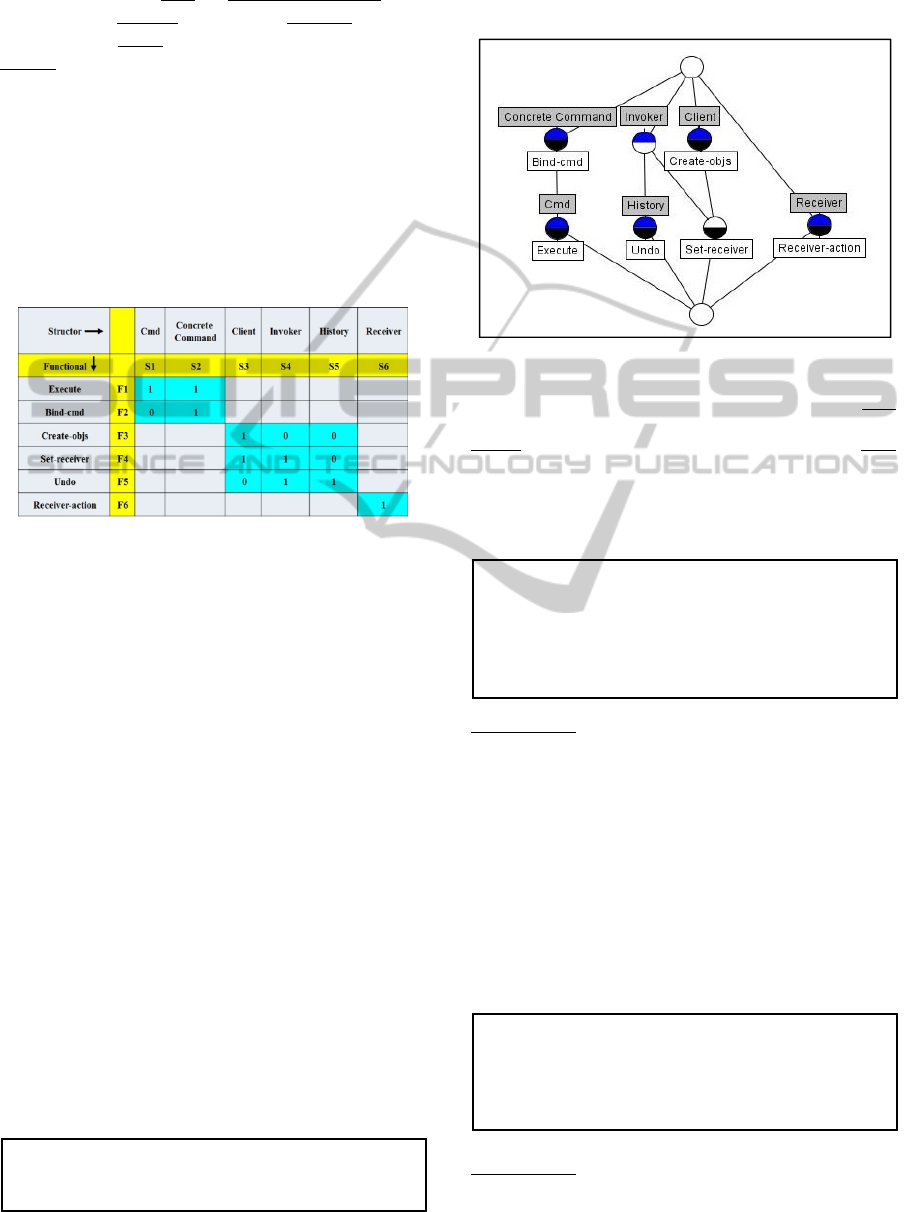
Block-diagonal modules, in Fig. 1, reflect the

pattern purpose: the command is decoupled from the

generic infrastructure. The top-left module is the

command itself, its abstract interface and concrete

implementation. The middle module is the generic

infrastructure: a client, the invoker and a history

mechanism for undo operations. The bottom-right

module is a specific receiver and its action.

Figure 1: Command Design Pattern Modularity Matrix.

It has six structors and functionals, forming three modules

(blue background): a- upper-left, the command; b- middle,

the generic infrastructure c- lower-right, the specific

receiver. Zeros outside modules are omitted for simplicity.

3.2 Command Modularity Lattice

We use the Modularity Matrix in Fig. 1 to generate

the Command Modularity Lattice. The result in Fig.

2, is obtained by the (Concept Explorer, 2006) tool.

4 THEORETICAL

CONSIDERATIONS

The set of Definitions and Theorems herein, for both

Modularity Matrix and Modularity Lattice, form

altogether the equivalence proof of these

representations regarding modularity.

4.1 Modularity Lattice Defined

We define a Modularity Lattice with respect to the

Modularity Matrix (Exman, Nov 2012):

Definition 1: Modularity Lattice

A Modularity Lattice is a conceptual lattice

generated from a Modularity Matrix.

A standard Modularity Lattice is generated from a

standard Modularity Matrix. From this definition

follow its characteristic properties.

Figure 2: Command Design Pattern Modularity Lattice -

Any path (or set of paths) from Top to Bottom not linked

to other paths is a module. One sees 3 modules: a- l.h.s.

with 2 attributes (Concrete Command and Cmd); b-

middle with 3 attributes (Client, Invoker, History) c- r.h.s.

with 1 attribute (Receiver). These match the matrix in Fig.

1. Nodes may have three colors: upper-half blue – an

attribute is associated with the node; lower-half black – an

object is associated with the node; white – no association.

Lemma 1: Standard Modularity Lattice

Properties

a- Its number of attributes is the same as its

number of objects;

b- No specific object is the Top; no specific

attribute is the Bottom.

Proof outline:

a- This property is obvious from the fact that the

Modularity Matrix is square;

b- This follows from the requirement that the

standard Modularity Matrix should not have

column vectors or row vectors fully consisting

of 1-valued matrix elements.

4.2 Modularity Lattice Modules

The Modularity Matrix modules are its diagonal

blocks. Modularity Lattice modules are given by:

Theorem 1: Modularity Lattice Modules

The modules of a software system in its

Modularity Lattice are the connected components

obtained when one cuts the Top and the Bottom

from the Modularity Lattice.

Proof outline:

Modules of a Modularity Matrix are diagonal

LinearSoftwareModels:EquivalenceofModularityMatrixtoItsModularityLattice

111

blocks whose set of structors and functionals are

disjoint from the respective sets of other modules.

Since structors correspond to Lattice attributes and

their functionals to the respective Lattice objects, a

set of attributes/objects disjoint to other sets has no

edges to other attributes/objects, except the Lattice

Top and Bottom. Cutting the latter from the Lattice

leaves a set of connected components corresponding

to the Modularity Matrix modules.

The converse of Theorem 1 is easily verified.

Next, we deal with different kinds of modules in

the Modularity Lattice. The paths in the next

corollary refer to connected components after

cutting edges to Top/Bottom of the Lattice.

Corollary: Modularity Lattice Module Types

1a- single path with single node – a path with no

edges to other paths, and a single node, fits a

purely diagonal Modularity Matrix module;

1b- single path with N nodes – a path without

edges to other paths, with N nodes, fits a block-

diagonal N-dimension module forming a full

lower triangular matrix in the block, in a

Modularity Matrix having no outliers.

1c- a set of connected paths – a set of paths with

edges among paths within the set, and N attributes

fits an N-dimension diagonal block, in a

Modularity Matrix having no outliers.

Proof outline:

1a- a single node means just one attribute with one

object;

1b- N nodes mean that there are N attributes, one

for each node, therefore also N objects, as the

module must be square; the full triangular

matrix within the block is needed to avoid

linear dependence among the structors in the

Modularity Matrix, since each attribute has all

the objects in its own node and below its node;

1c- N nodes mean that there are N attributes, one

for each node, therefore also N objects, as the

module must be square; since there are two or

more paths, not all attributes have all the

objects below its node in the same path.

It is straightforward to obtain module attributes

and objects in the Modularity Lattice, corresponding

to their Modularity Matrix. Going downwards (from

Top to Bottom) in any path, one uses set intersection

for objects, to obtain the respective objects of the

next node, down to one-level above the Bottom.

Going upwards in any path, one uses set intersection

for attributes, to obtain the respective attributes of

the next node, up to one-level below the Top. For

more details see e.g. (Belohlavek, 2008).

4.3 Modularity Matrix Outliers

Criterion

Formally within Linear Software Models, cohesion

is defined in terms of sparsity of the Modularity

Matrix (Exman, 2012). Sparsity of a matrix is the

ratio between the number of zero-valued elements to

the total number of elements in the matrix:

Sparsity = NumZeros/TotalNumElements (3)

In general, one expects the sparsity of modules

to be lower than the sparsity of the Modularity

Matrix elements outside the modules. Thus, the

lower is the sparsity, the higher the cohesion. This

implies a threshold of maximal sparsity inside a

module. For instance, assuming a maximal sparsity

threshold of 50%, one writes:

Module_Sparsity < 0.5

(4)

An outlier is a 1-valued matrix element in the

Modularity Matrix outside of any of the diagonal

blocks. Outliers are coined interferences in the

Conceptual Lattice domain (Lindig, 1997). Outliers

cause an undesirable coupling between modules.

The outcome of this coupling is a much larger

coupled diagonal block made of:

• The joint original diagonal blocks coupled by

the outliers;

• A few 1-valued matrix elements outside the

original blocks – the coupling outliers;

• Many zero-valued matrix elements surrounding

the outliers.

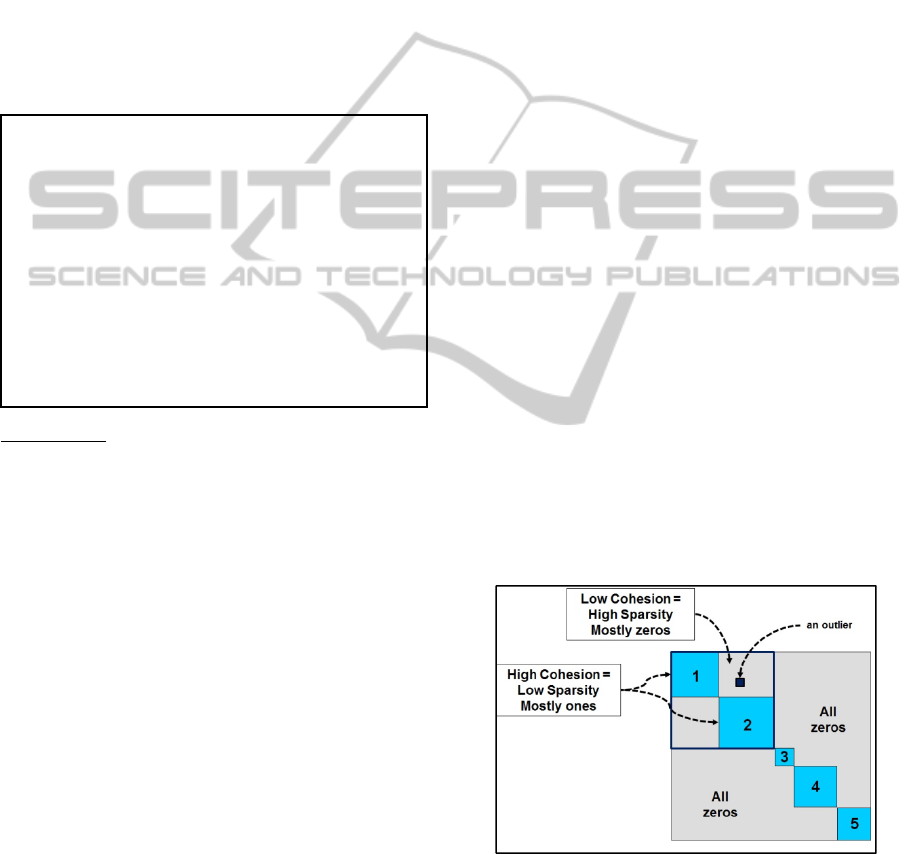
The resulting larger coupled diagonal block has

a much lower cohesion than the original modules

coupled by the outlier (see Fig. 3).

Figure 3: Block-diagonal Modularity Matrix with coupling

outlier – There are 5 original modules (marked by blue

background), all of them with high cohesion (i.e. low

sparsity). The outlier couples modules 1 and 2. Around the

outlier there are mostly zeros, causing high sparsity (i.e.

low cohesion) of the coupled joint module of 1 and 2.

ICSOFT-PT2015-10thInternationalConferenceonSoftwareParadigmTrends

112

Searching for outliers, outside the original

modules, the inequality sign is inverted, as the

sparsity is above the threshold:

Outlier_Sparsity_Criterion > 0.5

(5)

The TotalNumElements (total number of

elements) of a block in the Modularity Matrix is the

square of NumStructors, (number of structors). The

NumZeros (number of zero-valued matrix elements)

equals the TotalNumElements minus NumOnes

(number of 1-valued matrix elements). Substituting

these terms in equations (3) and (5), one finally gets

the Outlier Sparsity Criterion for the presence of

outliers in a coupled module of a Modularity Matrix:

Outlier_Sparsity_Criterion =

0.5 * (NumStructors)

- NumOnes > 0

(6)

4.4 Modularity Lattice Outliers

Criterion

To find the equivalent Outlier Sparsity Criterion for

a Modularity Lattice, we use the same previous

equation, substituting it with Lattice quantities:

Theorem 2: Modularity Lattice Outliers

Criterion

Given equation (6) for a Modularity Matrix, the

equivalent Outlier Sparsity Criterion for a

Modularity Lattice module containing outliers is

Outlier_Sparsity_Criterion =

0.5 * (NumAttributes)

- NumOnes > 0

where

NumOnes = LocalPairs + EdgePairs.

LocalPairs is the number of nodes in which there

are both an attribute and its object locally.

EdgePairs is the number of edges below each

attribute node needed to reach each of its objects,

down to the lowest object, above the Bottom.

Proof outline:

Given equation (6) above, then:

NumAttributes (Number of attributes) in a module is

trivially equal to NumStructors (Number of

structors). NumOnes (Number of 1-valued matrix

elements) is the number of links between attributes

(structors) and objects (functionals). These are of

two Attribute-Object Pair types: a- Local – both in

the same node; b- Edge – in different nodes linked

by edges. Thus, one only needs to count and sum

correctly both types of Attribute-Object pairs.

To illustrate the calculation of quantities

appearing in Theorem 2, we take the simple example

of the Command design pattern middle module. By

the Modularity Lattice in Fig. 2, the number of

Attributes is 3 (Client, Invoker and History). The

first term of the r.h.s. of the equation in Theorem 2

is half the square of NumAttributes, i.e. 4.5. The

second term NumOnes equals 5 which is the sum of

2 LocalPairs (Client/CreateObjs and History/Undo)

and 3 EdgePairs (edges from Invoker-to-Undo,

Invoker-to-Set-Receiver and Client-to-Set-

Receiver). As the Outlier_Sparsity_Criterion is

negative, there is no outlier in this module.

This calculation is totally equivalent to equation

(6). By the Modularity Matrix middle module in Fig.

1, the number of Structors is also 3 (Client, Invoker

and History). Half the square of NumStructors is

4.5. By directly counting the number of ones in the

middle module in Fig. 1, NumOnes equals 5. The

conclusion is the same: no outliers in this module.

5 HEURISTICS FOR

DECOUPLING

Once outliers were pointed out in a system design,

software engineers should apply their ingenuity to

solve the coupling problems and improve the design.

A heuristic rule suggests a decoupling starting

point. This rule is alternatively formulated either in

terms of the Modularity Matrix or in terms of the

Modularity Lattice.

Decoupling Heuristic Rule

Modularity Matrix version

Start decoupling with a row/column with a large

number of 1-valued (outlier) matrix elements.

Modularity Lattice version

Start decoupling with a Lattice node with a large

number of edges to other nodes.

In order to systematically eliminate outliers in a

Modularity Lattice, one should look first for the

node with a maximal connectivity to other nodes.

Then look for the next node in terms of connectivity,

and so on. Following the heuristic rule, a way to deal

with an outlier node coupling of potential modules

in the Modularity Lattice, is to erase a minimal

number of edges from the outlier node and see

whether this reduces the lattice to a modular one.

6 CANONICAL CASE STUDIES

Here we look at software systems case studies,

which are canonical from a modularity viewpoint.

These case studies have been analysed earlier,

LinearSoftwareModels:EquivalenceofModularityMatrixtoItsModularityLattice

113

(Exman, 2014), but here we show the equivalence of

the Modularity Matrix to the respective Lattice.

6.1 The Observer Design Pattern

The Observer design pattern is taken from the GoF

book (Gamma, 1995). Its well-known purpose is a

many-following-one behavior, viz. many observers

change according to the changes in the one subject.

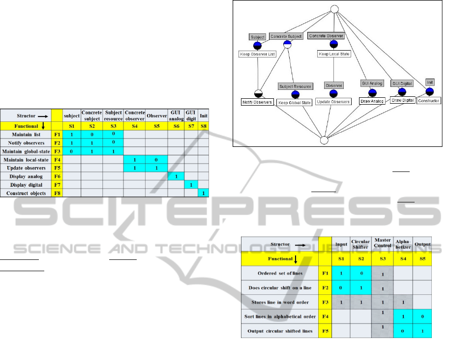
Figure 4: Observer Design Pattern Modularity Matrix.

There are 8 structors and functionals in this matrix.

These form 5 modules (in blue background): a-

upper-left subject role; b- middle observer role; c-

lower-right three strictly diagonal modules: specific

application GUIs and initiator.

The Observer structors are (abstract/concrete)

subject and observer, (analog/digital) clock

application GUI (Graphical User Interface), a

subject resource (the internal clock) and an initiator

to construct objects. The pattern functionals include

the clock application Display “digital” and “analog”.

The Observer Modularity Matrix in Fig. 4 shows

a perfect block-diagonal modularity. The upper left

block is the subject. The middle block is the

observer. The lower right structors refer to

application specific GUI and the initiator. The

corresponding Modularity Lattice is seen in Fig. 5,

following, from left to right, Module types 1c, 1b

and 1a of the Corollary in sub-section 4.2.

6.2 The Parnas KWIC System

Parnas described in his seminal paper (Parnas, 1972)

the KWIC system for producing an index containing

sentences circular shifted through all possibilities,

keeping word order, and alphabetically sorted.

KWIC illustrated the idea of modularity. Two

modularizations were suggested: one with couplings

and another with couplings resolved.

The KWIC system 1

modularization illustrates a

coupling case, seen in the Modularity Matrix in Fig.

6. Its matching Lattice is in Fig. 7. Both

representations lead to the same conclusions.

The Parnas 1

Modularity Matrix of the KWIC

Figure 5: Observer Design Pattern Modularity Lattice –

There are 5 modules in this lattice: a- l.h.s. with 3

attributes (Subject, Concrete Subject, Subject Resource) is

the Subject Role; b- middle with 2 attributes (Concrete

Observer, Observer) is the Observer Role; c- r.h.s. with 3

modules, each with just 1 attribute (two GUIs and one

Init). Modules correspond to the matrix in Fig. 4.

Figure 6: Parnas KWIC System 1

Modularization Matrix

– This Modularity Matrix shows coupling between two

potential modules (marked by light blue background). The

coupling outliers (marked by hatched background) are in

column S3 (the Master Control) and in row F3.

system in Fig. 6 points to two couplings (with a

hatched background): a- the Master Control is not a

real sub-system, as it refers to all functionals (a

whole column S3 of 1-valued matrix elements); b-

the “Store line in word order” functional in row F3

is a coupling of any two potential modules (marked

by a blue background).

The Parnas KWIC 1

modularization Modularity

Lattice in Fig. 7 points to exactly the same couplings

as its Modularity Matrix: a- The Master Control is

indeed not a real sub-system, as it appears at the Top

(its extent is all the 5 objects!); b- The node of the

“Stores line in word order” has no proper attribute

and it couples every attribute, except Output;

The solution of the above coupling problems is to

eliminate the Master Control from the system

composition as it is not a sub-system and add a new

“Line Storage” structor (attribute), to which all the

ICSOFT-PT2015-10thInternationalConferenceonSoftwareParadigmTrends

114

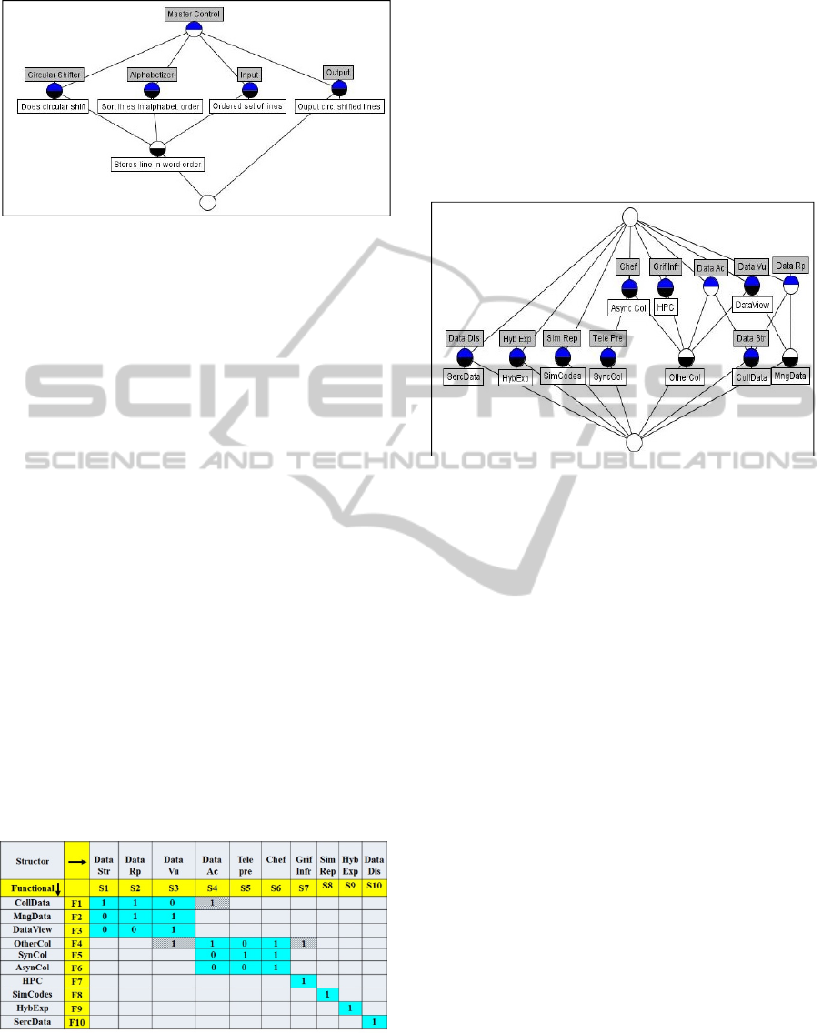
Figure 7: Parnas KWIC System 1

Modularization Lattice

– Two modules are apparent in this lattice: a- l.h.s. with 4

attributes (Circular Shifter, Alphabetizer, Input, Master

Control); b- r.h.s. with 2 attributes (Output, Master

Control). The Master Control couples the 2 modules. The

“Stores Line in word order” object is also coupling the

l.h.s. module. This Lattice matches the matrix in Fig. 6.

other structors refer for “Storing line in word order”.

The outcome fits Parnas KWIC 2

modularization which is indeed canonical. It is a

strictly diagonal Modularity Matrix, and a matching

Lattice with five neat single node modules.

7 REAL SYSTEM CASE STUDY

7.1 The NEESGrid System

This system, developed at the NCSA at Urbana,

Illinois, enables a “Network Earthquake Engineering

Simulation” – for details see (Finholt 2004).

The system Modularity Matrix is in Fig. 8. It

has three diagonal blocks. The top-left module refers

to Data as seen by structor and functional names.

The middle module refers, by the functionals with

Col suffix, to collaboration types, viz. synchronous,

asynchronous and other. The right bottom strictly

diagonal elements are external modules.

Figure 8: NEESGrid System Modularity Matrix – shows

coupling mainly between two 3*3 modules (with light

blue background). The coupling outliers (with hatched

background) are in column S4 (DataAc) and in row F4

(OtherCol).

Of the 3 outliers (with hatched background)

close to the block borders, two of them are in the

OtherCol row F4 and the third one in the DataAc

column S4, pointing out to specific couplings.

7.2 The NEESGrid Modularity Lattice

There is a clear matching between the NEESGrid

Modularity Matrix in Fig. 8 and its Lattice in Fig. 9.

Figure 9: NEESGrid Modularity Lattice – The three

groups of modules here are: a- the left group containing 3

one-attribute modules (DataDis, HybExp, SimRep); b- the

middle module with Col objects (SyncCol, AsynCol,

OtherCol); c- the right group with Data Attributes/Objects

(DataVu, DataRp, Data Str). OtherCol and DataAc are

couplings between the second and third modules.

The Modularity Lattice has 3 left-most paths

with just 1 node in each path, fitting the Modularity

Matrix purely diagonal elements.

The right-most group of modules in the

Modularity Lattice referring to Data, with attributes

DataVu, DataRp, DataStr, fits the Modularity Matrix

top-left module. The middle group of modules in the

Modularity Lattice refer to collaborations (Col)

having three objects SyncCol, AsyncCol, OtherCol.

But, these right-most and middle groups of

modules are coupled. This can be checked by

computing the Outlier Sparsity Criterion for these

coupled Modularity Lattice modules (from Theorem

2 in sub-section 4.4), which is 10.5. It is bigger than

zero thus there are outliers in these coupled modules.

The node with the OtherCol object has no

attribute by itself and is the most linked node in the

Lattice, thus a good starting point for decoupling

analysis. This agrees with the Modularity Matrix,

OtherCol F4 row with maximal outlier number.

Both representation analyses lead to the same

potential modules, and the same suspect outliers.

LinearSoftwareModels:EquivalenceofModularityMatrixtoItsModularityLattice

115

8 DISCUSSION

This work has shown by theoretical arguments and

case studies, the equivalence between two different

modularity representations of a software system, viz.

the Modularity Matrix and its Modularity Lattice.

This is interesting as it mutually reinforces their

independent conclusions, and it triggers new

questions in each representation, motivated by the

line of thoughts of the other one.

In practical terms, both representations enable to

assess modularity of a software system and to

highlight localized couplings deserving software

sub-system redesign.

8.1 Future Work

Concerning rigorous formalization, linearity still is

an open issue worth of investigation in the context of

Modularity Lattices. Moreover, is there any meaning

to non-linearity for software systems?

In the context of Modularity Matrices, we have

asked whether systems with outliers like the

NEESGrid system, are amenable to complete block-

diagonalization or they are essentially non-block-

diagonal. Are these systems the exception, or a class

on their own? The equivalence of Modularity

Matrices and Lattices should facilitate research.

REFERENCES

Baldwin, C.Y. and Clark, K.B., 2000. Design Rules, Vol.

I. The Power of Modularity, MIT Press, MA, USA.

Belohlavek, R., 2008. Introduction to Formal Concept

Analysis, Dept. of Computer Science, Palacky

University, Olomouc, Czech Republic.

Cai, Y. and Sullivan, K.J., 2006. Modularity Analysis of

Logical Design Models, in Proc. 21

IEEE/ACM Int.

Conf. Automated Software Eng. ASE’06, pp. 91-102,

Tokyo, Japan.

Concept Explorer, 2006 – Web site:

http://conexp.sourceforge.net/. Visited May 2015.

Exman, I., 2012. Linear Software Models for Well-

Composed Systems, in S. Hammoudi, M. van

Sinderen and J. Cordeiro (eds.), 7

ICSOFT’2012

Conf., pp. 92-101, Rome, Italy.

Exman, I., November 2012. Linear Software Models,

Extended Abstract, in I. Jacobson, M. Goedicke and P.

Johnson (eds.),. GTSE 2012, SEMAT Workshop on

General Theory of Software Engineering, pp. 23-24,

KTH Royal Institute of Technology, Stockholm,

Sweden,. See also video presentation:

http://www.youtube.com/watch?v=EJfzArH8-ls.

Exman, I., 2013. Linear Software Models are Theoretical

Standards of Modularity, in J. Cordeiro, S.

Hammoudi, and M. van Sinderen (eds.): ICSOFT

2012, Revised selected papers, CCIS, Vol. 411, pp.

203–217, Springer-Verlag, Berlin, Germany. DOI:

10.1007/978-3-642-45404-2_14.

Exman, I., 2014. Linear Software Models: Standard

Modularity Highlights Residual Coupling, Int. Journal

on Software Engineering and Knowledge Engineering,

vol. 24, pp. 183-210, March 2014. DOI:

10.1142/S0218194014500089.

Finholt, T.A., Horn, D. and Thome, S., 2004. NEESgrid

Requirements Traceability Matrix, Technical Report

NEESgrid-2003-13, University of Michigan.

Gamma, E., Helm, R., Johnson, R. and Vlissides, J., 1995.

Design Patterns: Elements of Reusable Object-

Oriented Software, Addison-Wesley, Boston, MA.

Ganter, B. and Wille, R., 1999. Formal Concept Analysis.

Mathematical Foundations. Springer.

Ganter, B., Stumme, G. and Wille, R., 2005. Formal

Concept Analysis - Foundations and Applications.

Springer.

Heckmann, P. and Speicher, D., 2012. Assisted Software

Exploration using Formal Concept Analysis”, in

SKY’2012 3

Int. Workshop on Software Knowledge,

pp. 11-21, SciTePress, Portugal.

Lindig, C. and Snelting, G., 1997. Assessing Modular

Structure of Legacy Code Based on Mathematical

Concept Analysis, in ICSE’97 Proc. 19

Int. Conf. on

Software Engineering, pp. 349-359, ACM. DOI:

10.1145/253228.253354.

Parnas, D.L., 1972. On the Criteria to be Used in

Decomposing Systems into Modules, Comm.. ACM,

15, 1053-1058.

Siff, M. and Reps, T., 1999. Identifying modules via

concept analysis, IEEE Trans. Software Engineering,

Vol. 25, (6), pp. 749-768. DOI: 10.1109/32.824377.

Snelting, G., 2000. Software reengineering based on

concept lattices, in Proc. of 4

European Software

Maintenance and Reengineering, pp. 3-10, IEEE.

DOI: 10.1109/CSMR.2000.827299.

Steward, D., 1981. The Design Structure System: A

Method for Managing the Design of Complex

Systems, IEEE Trans. Eng. Manag., EM-29 (3), pp.

71-74.

Wille, R., 1982. Restructuring lattice theory: an approach

based on hierarchies of concepts. In: I. Rival (ed.):

Ordered Sets, pp. 445–470, Reidel, Dordrecht-Boston.

ICSOFT-PT2015-10thInternationalConferenceonSoftwareParadigmTrends

116