
Spatio-Temporal Normalization of Data from Heterogeneous Sensors
Alessio Fanelli, Daniela Micucci, Marco Mobilio and Francesco Tisato
Department of Informatics, Systems and Communication University of Milano - Bicocca, Milan, Italy
Keywords:
Sensor Heterogeneity, Modularisation, Software Architecture, Knowledge Representation.
Abstract:
The growing use of sensors in smart environments applications like smart homes, hospitals, public transporta-
tion, emergency services, education, and workplaces not only generates constantly increasing of sensor data,
but also rises the complexity of integration of heterogeneous data and hardware devices. In order to get more
accurate and consistent information on real world events, heterogeneous sensor data should be normalized.
The paper proposes a set of architectural abstractions aimed at representing sensors’ measurements that are
independent from the sensors’ technology. Such a set can reduce the effort for data fusion and interpretation.
The abstractions allow to represent raw sensor readings by means of spatio-temporal contextualized events.
1 INTRODUCTION
Smart environments are usually instrumented with
various typologies of sensors. Sensors may have a
fixed position, like a thermometer or a light sensor,
or they may move inside the environment, like the
sensors embedded in smartphones. Moreover, sen-
sors are heterogeneous, thus producing measurements
that are semantically linked to their sources. Appli-
cations that rely on sensors’ measurements usually
fall under the umbrella of Ambient Intelligence (AmI)
that includes specific domains like smart homes,
health monitoring and assistance, hospitals, trans-
portation, emergency services, education, and work-
places (Cook et al., 2009). Such applications often are
required to know the specific device that originated
the measurement in order to understand and use the
information provided. This leads to vertical systems,
which feature low modularity and scarce openness.
When modeling sensors and related measure-
ments, architectural solutions should face the chal-
lenge related to both heterogeneity and semantics. For
example, authors in (Widyawan et al., 2012) propose
a layered architecture that provides the low-level soft-
ware, the middleware, and the upper-level services
with detailed specifications of the involved sensors.
This way sensors are well modeled, but their knowl-
edge is distributed throughout all the system. Authors
in (Dasgupta and Dey, 2013) focus on issues related
to the management of large amount of data from sen-
sors: the proposed approach consists in transforming
sensor data in what authors call a set of observations
that are meaningful for the applications. Lower lev-
els embed semantics that is strictly related to the spe-
cific application. This lead to scarce reusability as the
same abstraction rules for a specific sensor may not
be applicable in different contexts. Finally, database
approach is growing interest. Indeed, the database ap-
proach allows heterogeneous applications to access
the same sensor data via declarative queries. This
kind of solutions may resolve data heterogeneity at
the application level, but there still persists the issue
of sensor data management, since most of the exist-
ing solutions suppose homogeneous sensors generat-
ing data according to the same format (Gurgen et al.,
2008).
The identification of a suitable set of architec-
tural abstractions, able to represent sensor measure-
ments independently from the hardware characteris-
tics of the source, could improve reusability, open-
ness, and modularity of software systems. These
abstractions allow to remove the dependency from
the sensor by contextualizing the measurements in
a spatio-temporal frame. Measurements result in
spatio-temporal events that can be stored inside a
Data Base Management System (DBMS) or streamed
inside a Data Stream Management System (DSMS)
(Motwani et al., 2002), as proposed in (Gurgen et al.,
2008). The main benefit is that applications no longer
need to know the kind and the numbers of deployed
sensors. Upon the occurrence of an event of interest,
applications can decide to access all the other events
that are related both spatially and temporally. In this
paper neither the storage nor distribution of data is
462
Fanelli A., Micucci D., Mobilio M. and Tisato F..
Spatio-Temporal Normalization of Data from Heterogeneous Sensors.
DOI: 10.5220/0005559504620467
In Proceedings of the 10th International Conference on Software Engineering and Applications (ICSOFT-EA-2015), pages 462-467
ISBN: 978-989-758-114-4
Copyright
c
2015 SCITEPRESS (Science and Technology Publications, Lda.)

handled, but the focus is on the definition of such a
set of architectural abstractions that could solve sen-
sors heterogeneity issue, in order to be able to apply
one of the mentioned approaches for data distribution,
storage, and usage.
This paper will present the basic concepts along
with the following simplified case of study. Con-
sider a smart building composed by different rooms;
in each room different sensors are located. In our ex-
ample, we consider a room only (room1) that is in-
strumented as follow: in the top corner there is a cam-
era (cam1) facing the centre of the room. Hanged on
the wall there is also a thermometer (therm1). More-
over, a person in the room owns a smartphone with the
accelerometer acc1. In this kind of contexts, smart-
phones are usually considered as extensions of the
user, which means that their position is the same. Sev-
eral applications can rely on the above listed sensors:
a tracking application could try to follow the user (ei-
ther a specific one or any user) and could make the
position available to the system; an application could
exploit the locations of the users to control the temper-
ature in the rooms accordingly, based on their needs
or preferences. These are just a few examples that can
benefit from the proposed approach.
The rest of this paper is organized as follow: Sec-
tion 2 introduces the basic concepts used to model
spatial contextualization; Section 3 presents the pro-
posed abstractions; finally Section 4 sketches some
final remarks about the ongoing work and provides
details about the future directions.
2 BACKGROUND CONCEPTS
Spatial contextualization has been derived from con-
cepts defined in (Tisato et al., 2012; Micucci et al.,
2014) and that will be summarized in the following.
A space is a set of potential locations, that are all
the locations that could be theoretically considered in
that space. For example, in a graph the potential loca-
tions are all the nodes. On the other hand, if a Carte-
sian space is used to localize entities within a room,
then the potential locations are every point in R
2
of
the area delimited by the room perimeter. Applica-
tions explicitly manage effective locations, which are
a subset of space’s potential locations. For example,
an application that calculates the trajectory of a mo-
bile entity will only explicitly consider a finite number
of locations in the Cartesian space, that is, the loca-
tions belonging to the trajectory.
A zone C
S
is a subset of potential locations of a
space S. It is defined by a set of effective locations
termed characteristic locations in S and by a member-
ship function that states if a given location of S be-
longs to the zone. Essentially, the membership func-
tion is a boolean function that is true when a loca-
tion falls within the zone. According to the member-
ship function used, different kinds of zones can been
identified, such as: enumerative, premetric declara-
tive, polygonal, and pure functional. We focus on the
pure functional type. Figure 1 shows the concepts of
space, zone, location and membership function.
Zone
MembershipFunction
+ belongsTo(location) :boolean
Location
Space
1
+effective 1..*
+characteristic
*
1
defined over
1
Figure 1: Space, Location, and Zone.
Given two different zones, a mapping relation is
a generic function defined in C
S
1
− > C
0
S
2
(where S
1
and S
2
are spaces, and C
S
1
and C
0
S
2
are zones defined
on those spaces respectively). Thus it can be seen as
a mapping between zones in different spaces.
Space MappingRelation
+ map(Zone) :Zone
+source
1
+reference
1
Figure 2: Mapping Relation.
Figure 2 pictures the concept of mapping relation
with one of the spaces acting as reference space, so it
can be seen in a hierarchical fashion with hierarchies
of spaces mapped through mapping relations.
3 THE MODEL
Measurements from sensors can be modeled as data
contextualized in a spatial-temporal context. Time
contextualization is not detailed here for shortness.
Concepts related to time and to clocks synchroniza-
tion can be found in (Fiamberti et al., 2012). Before
describing the model in detail, an overall presentation
will be provided.
3.1 General Overview
The approach proposes an abstraction process able to
produce spatio-temporal contextualized events, start-
ing from low level measurements that are strictly sen-
sor dependant.
Figure 3 provides a graphical representation of the
identified abstractions: at the bottom level there are
Spatio-TemporalNormalizationofDatafromHeterogeneousSensors
463
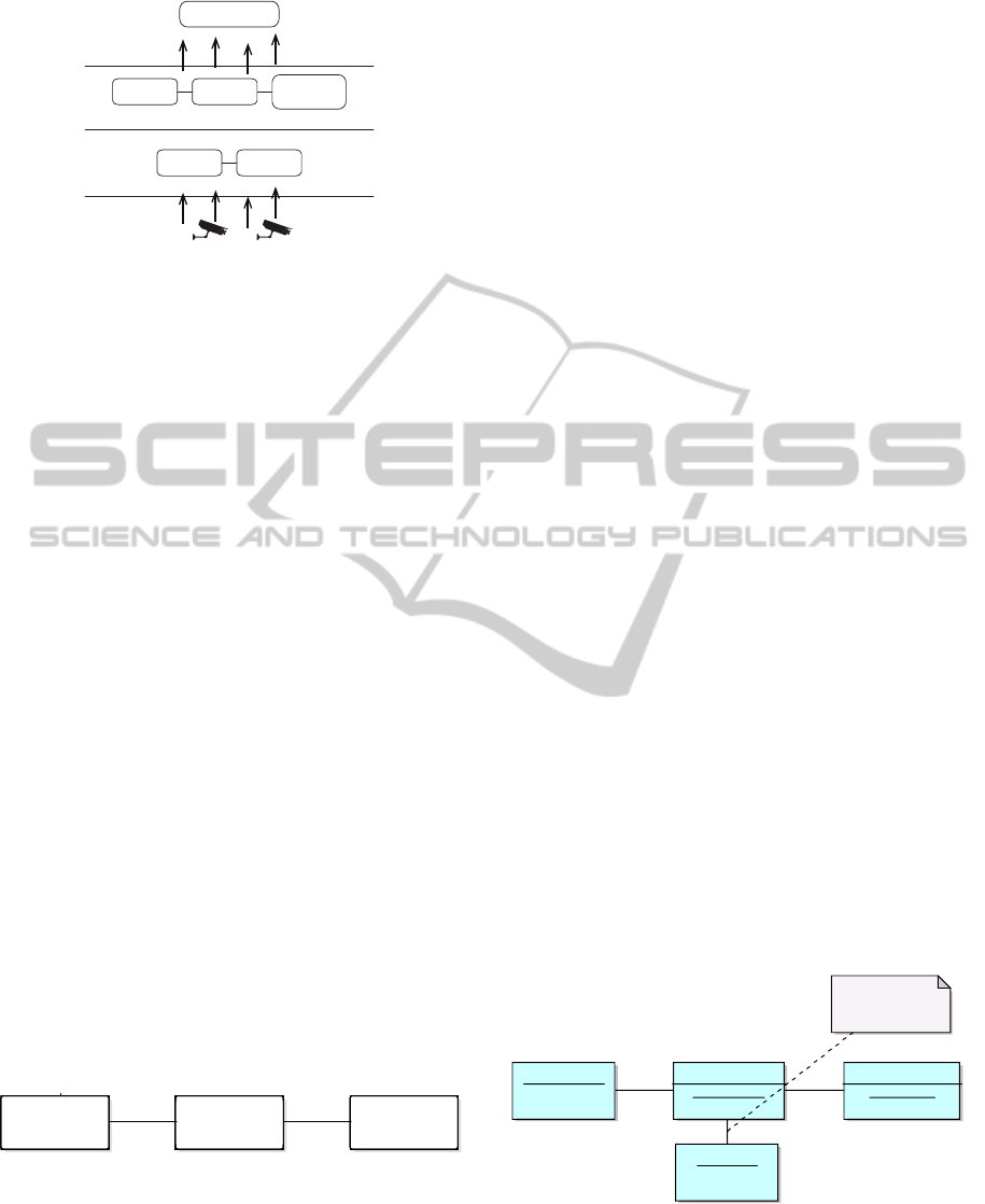
Sensor
Data
Normalized Stimuli Level
Stimuli Level
Signals
Applications
Time
Data
Zone
Space
Figure 3: Abstractions.
physical sensors, which are considered outside the
system. Sensors produce signals that are here in-
tended as raw samplings. Raw sampling is then ab-
stracted into stimuli, which are the lower level infor-
mation the system receives and that is strictly related
to its hardware source. In Figure 3, stimuli are de-
picted at the stimuli level and are represented by data
associated to sensors. At the normalized stimuli level,
stimuli are contextualized both spatially and tempo-
rally and are denoted normalized stimuli. For spatial
contextualization we intend that the stimulus (data in
Figure 3) has associated a zone in a space that models
the physical environment. For temporal contextual-
ization we intend that all the stimuli have associated a
time value that is related to the same clock. This way,
all the stimuli are contextualized in the same refer-
ence frames (time and space) and can be viewed by
the applications as events occurred in specific places
in the physical environment at specific time instants
relieving them by low level and hardware dependent
details.
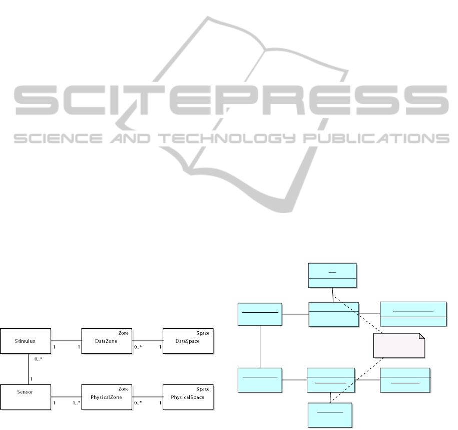
3.2 Sensors
Sensors are the meta representation of the physical
sensors; they are in charge of acquiring signals and
providing stimuli. As shown in Figure 4, sensors are
localized in a physical space (PhysicalSpace)
through a physical zone (PhysicalZone).
PhysicalSpace and PhysicalZone are special-
ization of Space and Zone respectively as defined in
(Tisato et al., 2012; Micucci et al., 2014).
Stimulus
Sens or
Zone
Phys icalZone
Space
Phys icalS pace
Zone
DataZone
Space
DataSpace
1
0.. *
1 1.. * 0.. * 1
1 1 0.. * 1
Figure 4: A sensor and its physical localization.
A physical space is a space that models the ac-
tual physical world; it is used to localize entities (and
events also). A special class of entities are the sen-
sors.
Localization means placing an entity in a well de-
fined position inside the physical space. This can be
achieved by using zones as defined in (Tisato et al.,
2012; Micucci et al., 2014) and introduced in Section
2. This may suffice when the orientation of a sensor
does not affect the interpretation of the acquired val-
ues. For example, the measurements of a temperature
sensor are not affected by the orientation of the sensor
itself. On the other hand, such a definition may be too
poor. For example, consider a physical space as rep-
resented by a Cartesian 3D space with locations mod-
eled as a triple (x, y, z). A camera may be localized
through a zone that includes a characteristic location
with values for x, y, and z equal to the real position
in the world. Such localization is not sufficient to in-
terpret the acquired frames as the orientation is also
required. To fulfill this need, the concept of oriented
physical zone has been introduced as a specialization
of the physical zone, that also features the orientation,
in order to give a more consistent representation of a
position within a physical space.
Both physical space and corresponding locations
are specialized in order to model specific spaces ty-
pologies (e.g., 3D Cartesian, 2D grid, and so on) and
location typologies (e.g., a point in a 3D cartesian
space, a cell in a 2D grid, and so on). Zones are
not specialized because what characterizes a zone is
its membership function that can model, for instance,
cones, discretized spheres, and so on.
Considering the scenario introduced in Section 1,
room1 is represented by a 3D Cartesian space (a phys-
ical space). Suitable locations for this kind of space
are 3D points. Several kind of physical zones can be
defined over this space: single location zone, single
location oriented zone, cone zone, sphere zone. Ther-
mometer therm1 is localized inside room1 by means
of a physical zone constituted by a single location
that suffices to physically localize the acquired stim-
uli. Being sensor therm1 in position (0.3, 0.4, 0.1),
then, the characteristic location of its physical zone is
a 3D point with values [0.3, 0.4, 0.1] (see Figure 5).
therm1 :Sensor therm1PhysicalZone :
PhysicalZone
room1PhysicalSpace :
Cartesian3D
p1 :Point3D
indirect via Membership
function
Figure 5: Therm1 physical localization.
Camera cam1 has similar features: its position is
an oriented physical zone that represents the corner of
the room where it is fixed and the fact that is facing
the center of the room. Finally, accelerometer acc1
ICSOFT-EA2015-10thInternationalConferenceonSoftwareEngineeringandApplications
464
inside the smartphone is associated with the oriented
physical zone occupied by the smartphone itself. In
this case, the orientation represents how the smart-
phone is placed with respect to the room space, such
information is fundamental in order to correctly inter-
pret acc1’s data in most of domain applications (such
as dead reckoning).
3.3 Stimuli
Signals are raw data sensed (and usually sampled) by
sensors. Physical sensors emit signals, which are usu-
ally in form of voltages values. These signals are then
translated into stimuli through well-known conversion
functions. As an example, a simple temperature probe
is physically designed to output a voltage signal that
is linearly proportional to the local temperature. In
this example, the conversion function is the expres-
sion that maps such voltage readings into values that
represent the temperature in degrees.
Stimuli are referred to the sensor that produced
them and they are contextualized in zones (data
zones) of a specific space “owned” by the sensor: the
data space. A data space represents the admitted val-
ues for the sensor’s stimuli. For example, the data
space of an accelerometer is a 3D Cartesian space,
where the axes represent the ones of the acceleration
data and are in m/s
2
. It could have, as an example, a
valid range of + or - 4g. Locations in that space are
triples of values.
Data zones are simply zones defined in data
spaces. For example, a stimulus from an accelerom-
eter is located in a data zone whose characteristic lo-
cation is a location whose values corresponds to the
value read for each axis. If the stimulus is [x=0, y=1,
z=1], then the characteristic location of the data zone
is exactly [x=0, y=1, z=1].
Figure 6: Stimulus.
Figure 6 depicts the stimulus. It is associated to
the sensor that acquired its corresponding signal and
it is spatially contextualized by means of a data zone
(whose value equals the value of the sample) in the
sensor data space. Being data space a specialization
of space, it can be specialized like the physical zone to
represent different kind of data space (e.g., Fahrenheit
space, Celsius space, accelerometer space, and so on).
The same holds for its locations.
It is worth noting that the distinction between
physical space and data space and between physical
zone and data zone is purely conceptual: they are all
spaces and zones respectively as defined in (Tisato
et al., 2012; Micucci et al., 2014).
In the example scenario previously introduced,
there are three different types of stimuli. A sample
from therm1 is pictured in Figure 7. Sensor therm1
generates stimuli in a Celsius format. Thus, the sensor
data space is a Celsius temperature space that repre-
sents the space of the temperature readings by therm1
and whose locations are simply values in the scale (-
40 +40). A data zone for this kind of space includes a
membership function with associated one character-
istic location only. Suppose that therm1 acquires a
stimulus with value 23 Celsius Degree, then the l1
value is 23. Moreover, the stimulus temp1 is associ-
ated to therm1 sensor so that the information related
to the position of the sensor can be obtained.
A stimulus from cam1, instead, is localized via a
data zone in a image data space that represents the
space of the frames acquirable from cam1. The zone
has associated a set of locations that corresponds to
the matrix of the sensed image. Moreover, it is asso-
ciated the sensor cam1. Finally, an acceleration stim-
ulus from acc1 is localized in a data zone whose as-
sociated location corresponds to the sensed acceler-
ation. Such a zone is defined on a acceleration data
space that is a three dimensional space. Moreover, it
is associated to the sensor acc1.
temp1 :Stimulus
therm1 :Sensor
tempNZone :DataZone
therm1PhysicalZone :
PhysicalZone
l1 :
TemperatureLocation
indirect via Membership
function
room1PhysicalSpace :
Cartesian3D
p1 :Point3D
thermDataSpace :
FahrenheitTemperatureSpace
Figure 7: Stimulus Example.
3.4 Normalized Stimuli
A normalized stimulus is a further abstraction of a
stimulus and is depicted in Figure 8. It represents the
sensed value from a sensor that is spatially and tem-
Spatio-TemporalNormalizationofDatafromHeterogeneousSensors
465
porally contextualized and that is unrelated from the
sensor that produced it.
The normalization process takes into account the
physical position of the sensor and its characteristics,
in order to provide a physical zone in which the stim-
ulus is located and that is referred to the same phys-
ical space in which the source sensor is immersed.
Moreover, a normalized stimulus is located through
a normalized data zone in normalized data space. For
example, imagine that there are different temperature
sensors: some of them acquires in Celsius and others
in Fahrenheit. A normalized data space in this case
can be a Celsius data space in which localizing all the
temperatures.
Data
NormalizedStimulus
DataZone
NormalizedDataZone
DataSpace
NormalizedDataSpace
Space
PhysicalSpace
Zone
PhysicalZone
1
11
1
Figure 8: Normalized Stimulus.
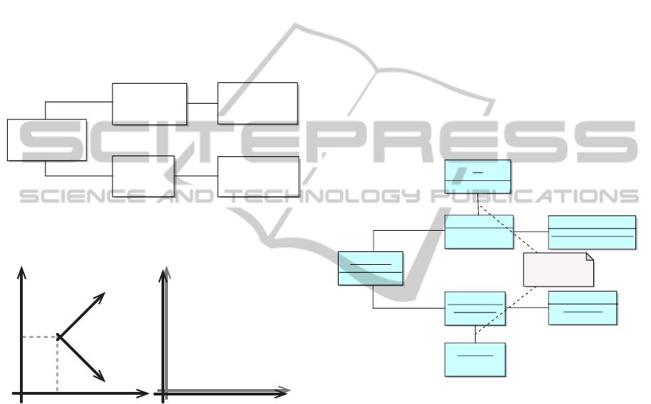
More complicated situations may occur.
Room PhysicalSpace
Sensor
Accelerometric DataSpace
(a)
Room
Accelerometric DataSpace
Room PhysicalSpace
(b)
Figure 9: Physical and Data Spaces relationships.
For example, Figure 9 shows the different rela-
tionships between a specific sensor’s data space, and a
normalized data space associated with a more broaden
and generic sensor. The room physical space repre-
sents the physical space of the room in which the sen-
sor is positioned (and oriented), while the sensor ac-
celerometric data space represents the data space of
the accelerometer values. As shown in Figure 9a, the
two spaces are not aligned: in this example an ori-
ented physical zone is required to consistently repre-
sent the position of the accelerometer inside the room
physical space. The orientation of the sensor will be
used as a parameter by the mapping relation function
that will translate the starting data zone into its nor-
malized counterpart, which will be related to the room
accelerometeric data space shown in Figure 9b. For
example, if the sensor is in the position showed in Fig-
ure 9a, the gravitational acceleration would be sensed
among both the axes of the sensor, while the normal-
ized value would only feature a −1g on the y axis.
Considering the example scenario, the previ-
ously defined temp1 stimulus depicted in Figure
7 was contextualized inside the thermDataSpace
data space and was expressed in Celsius degrees.
The corresponding normalized stimulus, as pic-
tured in Figure 10 will be contextualized inside the
tempNormalizedDataSpace, which, in this scenario
contains temperature readings in Fahrenheit degrees,
giving a good example of data zone normalization
in order to be globally consistent with all the other
homogeneous information source inside the room.
Moreover the normalized stimulus is localized inside
the physical space of room1 (room1PhysicalSpace).
Since the sensor was not oriented and its data has no
particular positioning, the position of the sensor and
of the normalized stimulus are in this case equivalent.
Temp1Norm :
NormalizedStimulus
tempNZone :DataZone
temp1NormZone :
PhysicalZone
room1PhysicalSpace :
Cartesian3D
tempNormalizedDataSpace :
CelsiusTemperatureSpace
p2 :Point3D
Indirect via Membership
function
l2 :
TemperatureLocation
Figure 10: Normalization Example.
The stimulus from cam1 needs a bit more of com-
putation in normalizing the oriented physical zone of
cam1 into the non-oriented physical zone in which the
normalized stimulus will be located. While the first
represents the position of the camera (a single point,
or a small well defined region of the physical space)
and its orientation, the latter in order to be represen-
tative for the normalized stimulus must represent the
physical cone viewed by cam1.
The normalization of the accelerations is similar
to the temperatures: the acceleration data zone, re-
ferred to the acceleration data space is normalized and
become a normalized acceleration zone in the room1
accelerations data space (i.e., the data space in which
all of the accelerations sensed in the room are contex-
tualized). The acceleration is also enriched with its
physical zone, which is a non-oriented physical zone
derived from the oriented physical one of acc1.
ICSOFT-EA2015-10thInternationalConferenceonSoftwareEngineeringandApplications
466

3.5 Data Flow
In Section 3.3 and 3.4 stimuli and normalized stimuli
have been defined. This subsection deals with how
those normalization happens. In Section 2 the concept
of mapping relation has been introduced: normalizing
a physical zone into another physical zone can be triv-
ial or quite complex depending on the nature of the
data, but it should always be a repeatable and deter-
ministic process, which means that it is possible to de-
fine a mapping function that relates any physical zone
into a corresponding physical zone in the reference
space. As already mentioned, the difference between
data and physical is purely logical, so it is reasonable
to say that data zones are normalized accordingly; it is
nonetheless noteworthy that a mapping relation could
easily need further information about the zones that
need to be normalized.
Using mapping relations in order to remove any
relationship between a sensor and the data it produces
allows to obtain homogenous data, resolving one of
the main issues of sensor heterogeneity.
Consider the acceleration previously defined and
normalized in the reference scenario. The physical
normalization is trivial and only consists in contex-
tualizing the stimulus in the non-oriented part of the
acc1 physical zone. The data zone conversion in-
stead, must use the orientation from the physical zone
of acc1 in order to normalize the acceleration from
the accelerations data space of acc1 to the room1 ac-
celerations data space that is jointly placed with the
room1 physical space: this means that, apart from
the usual conversions of scales and measurement unit,
a roto-translation of the acceleration is needed. The
information needed for this particular transformation
is the orientation of the accelerations data space of
acc1, which directly depends on the orientation of
acc1 itself. This is why acc1 has an oriented physi-
cal zone and its normalized stimuli does not: the ori-
entation has already been taken into consideration for
normalizing the acceleration data.
Similarly, the cam1 stimuli are normalized into
normalized stimuli that feature non-oriented physical
zones. This time the orientation is not used to manip-
ulate the data zone, but it is required, along with other
intrinsic parameters of cam1, to determine the shape,
size and displacement of the cone that represents the
physical zone of each normalized stimulus.
4 CONCLUSIONS
The proposed model has been implemented in a pre-
liminary proof-of-concept Java-based version in order
to test the main ideas. The testing has been conducted
exploiting simulated sensors, in particular accelerom-
eters and thermometers.
While a solid and wider implementation is re-
quired, the approach has proven to be effective and,
in the test case, efficient.
The main future directions include the manage-
ment of other typologies of senors including cameras;
an experimentation with real world sensors; and the
realization of data-flow mechanisms that domain ap-
plications can exploit to access and query normalized
stimuli.
REFERENCES
Cook, D. J., Augusto, J. C., and Jakkula, V. R. (2009).
Ambient intelligence: Technologies, applications, and
opportunities. Pervasive and Mobile Computing,
5(4):277 – 298.
Dasgupta, R. and Dey, S. (2013). A comprehensive sen-
sor taxonomy and semantic knowledge representa-
tion: Energy meter use case. In Sensing Technol-
ogy (ICST), 2013 Seventh International Conference
on, pages 791–799. IEEE.
Fiamberti, F., Micucci, D., Morniroli, A., and Tisato, F.
(2012). A model for time-awareness, volume 112 of
Lecture Notes in Business Information Processing.
Gurgen, L., Roncancio, C., Labb
´
e, C., Bottaro, A., and
Olive, V. (2008). Sstreamware: a service oriented
middleware for heterogeneous sensor data manage-
ment. In Proceedings of the 5th international con-
ference on Pervasive services, pages 121–130. ACM.
Micucci, D., Vertemati, A., Fiamberti, F., Bernini, D., and
Tisato, F. (2014). A spaces-based platform enabling
responsive environments. International Journal On
Advances in Intelligent Systems, 7(1 and 2):179–193.
Motwani, R., Widom, J., Arasu, A., Babcock, B., Babu, S.,
Datar, M., Manku, G., Olston, C., Rosenstein, J., and
Varma, R. (2002). Query processing, resource man-
agement, and approximation ina data stream manage-
ment system. Technical Report 2002-41, Stanford In-
foLab.
Tisato, F., Simone, C., Bernini, D., Locatelli, M. P., and
Micucci, D. (2012). Grounding ecologies on multiple
spaces. Pervasive and Mobile Computing, 8(4):575–
596.
Widyawan, Pirkl, G., Munaretto, D., Fischer, C., An, C.,
Lukowicz, P., Klepal, M., Timm-Giel, A., Widmer, J.,
Pesch, D., and Gellersen, H. (2012). Virtual lifeline:
Multimodal sensor data fusion for robust navigation in
unknown environments. Pervasive and Mobile Com-
puting, 8(3):388–401.
Spatio-TemporalNormalizationofDatafromHeterogeneousSensors
467
