
Exploring Machine Learning Techniques for Identification of Cues
for Robot Navigation with a LIDAR Scanner
Aj Bieszczad
Channel Islands, California State University, One University Drive, Camarillo, CA 93012 U.S.A.
Keywords: Mobile Robots, Navigation, Cue Identification, Machine Learning, Clustering, Classification, Neural
Networks, Support Vector Machines.
Abstract: In this paper, we report on our explorations of machine learning techniques based on backpropagation neural
networks and support vector machines in building a cue identifier for mobile robot navigation using a LIDAR
scanner. We use synthetic 2D laser data to identify a technique that is most promising for actual
implementation in a robot, and then validate the model using realistic data. While we explore data
preprocessing applicable to machine learning, we do not apply any specific extraction of features from the
raw data; instead, our feature vectors are the raw data. Each LIDAR scan represents a sequence of values for
measurements taken from progressive scans (with angles vary from 0° to 180°); i.e., a curve plotting distances
as a functions of angles. Such curves are different for each cue, and so can be the basis for identification. We
apply varied grades of noise to the ideal scanner measurement to test the capability of the generated models
to accommodate for both laser inaccuracy and robot motion. Our results indicate that good models can be
built with both back-propagation neural network applying Broyden–Fletcher–Goldfarb–Shannon (BFGS)
optimization, and with Support Vector Machines (SVM) assuming that data shaping took place with a [-0.5,
0.5] normalization followed by a principal component analysis (PCA). Furthermore, we show that SVM can
create models much faster and more resilient to noise, so that is what we will be using in our further research
and can recommend for similar applications.
1 INTRODUCTION
Automated Intelligent Delivery Robot (AIDer; shown
in Figure 1) is a mobile robot platform for exploring
autonomous intramural office delivery (Hilde et al.,
2009; Rodriguez et al., 2007). The research reported
in this paper was part of the overall effort to explore
ways to deliver such functionality. The robot was to
navigate in a known environment (a map of the
facility is one of the elements of AIDer’s
configuration) and carry out tasks that were requested
by the users through a Web-based application. Each
request included the location of a load that was to be
moved to another place that was also specified in the
request. The pairs of start and target locations were
entered into a queue that was managed by a path
planning module. When the next job from the queue
was selected, the robot was directed first to the start
location where it was to get loaded after announcing
itself, and then to the destination where it was to get
unloaded after announcing its arrival. That routine
was to be repeated indefinitely — if there were other
requests waiting in the queue and as long as there was
power.
Figure 1: Robot with a laser scanner (between the front
wheels).
645
Bieszczad A..
Exploring Machine Learning Techniques for Identification of Cues for Robot Navigation with a LIDAR Scanner.
DOI: 10.5220/0005569006450652
In Proceedings of the 12th International Conference on Informatics in Control, Automation and Robotics (ANNIIP-2015), pages 645-652
ISBN: 978-989-758-122-9
Copyright
c
2015 SCITEPRESS (Science and Technology Publications, Lda.)
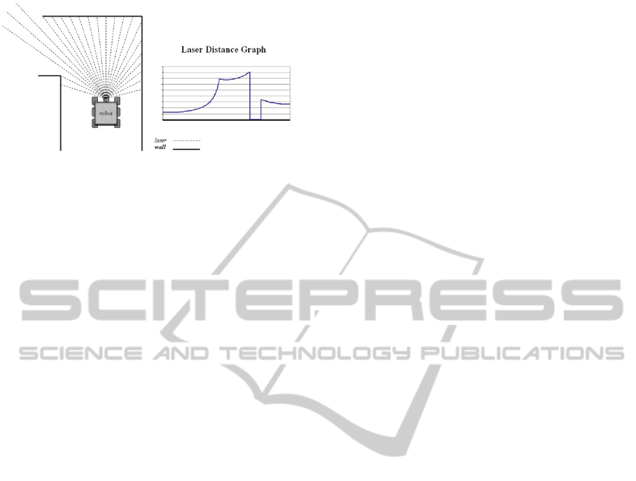
Figure 2: Robot with a rotating laser scanner (between the
front wheels) generates a sequence of distances for each
progressive angle.
One of the major objectives was to provide the
functionality at low cost. Therefore, AIDer has a very
limited set of sensors for navigation: right side
detectors of the distance from the wall, and a frontal
2D (one-plane) LIDAR laser scanner for detecting
cues such as turns and intersections. The side sensors
are used to provide a real-time feedback to a
controller that corrects the position of the robot so it
stays at a constant distance from the right wall (Hilde
et al., 2007).
Higher-level navigation in AIDer is based on
following paths that consist of a series of intervals
between landmarks (Rodriguez et al., 2007). A map
of the facility is provided as an element of the
configuration (using a custom notation), so the robot
is not tasked with mapping the environment. The map
configuration file includes locations of landmarks
along with exact distances between the landmarks.
Upon receiving the next task to carry out, the robot
determines the path to travel in terms of the
landmarks. The path is divided into a sequence of
landmarks, and the robot is successively directed to
move to the next landmark. After the current target
landmark is identified, the robot receives the next
target landmark to go to. To accommodate for error
in mobility (like slippage of the wheels) that may
skew the robot orientation based purely on traveling
exact distances, the robot relies on identification of
cues to verify reaching landmarks.
In an environment lacking GPS, identification of
environmental cues is a critical low-level task
necessary for recognizing landmarks (Thrun, 1998),
since landmarks are defined in terms of cues. The
frontal laser-scanner in AIDer serves that purpose.
Each scan produces a sequence of measurements that
differ depending on the shape of the surrounding
walls. For example, Figure 2 shows a scan of a left
turn. The scan results - a sequence of numbers
representing the measured distance (e.g., in inches) -
are graphed using angles on the x axis and the
distances on the y axis. Due to the range limitations
of the laser scanner, certain measurement may be read
as zeros; that is visible as a sudden drop in the curve
shown in the figure.
In (Hilde et al., 2007), an approach similar to
(Hinkel et al, 1988) was taken with a selective subset
of measurements used to define cues analytically with
a limited success.
In this paper, the complete raw set is used for this
purpose as will be shortly explained. Our earlier
attempts to use raw data in such a way were not
completely successful (Henderson, 2012), and the
research reported here remedies that.
2 RELATED WORK
Mapping and localization services are the foundation
of autonomous navigation (Thrun, 1998). As we
already stated, mapping is not a functional objective
of the AIDer. Vast majority of the current localization
work is based on utilization of very sophisticated
equipment as seen in cars participating in R&D
efforts in academia, auto industry, and government-
sponsored contests (e.g., Peters et al., 2008). Utilizing
simple sensors with very limited capabilities started
the field (Borenstein, 1997), but currently it’s rare to
depend on just such limited functionality. Yet, the use
of inexpensive devices is important in environments
lacking access to powerful computers or abundant
power supplies (e.g., Roman et al., 2007), and when
cost is a concern (e.g., Tan et al., 2010).
LIDAR-based identification was successfully
solved by analytical methods in (Hinkel et al, 1988)
in which histograms of laser measurements were used
as the input data. There have been numerous attempts
to use similar data using a variety of analytical
approaches (e.g., Zhang et al., 2000; Shu et al., 2013;
Kubota et al., 2007; Nunez et al., 2006).
(Vilasis-Cardona et al., 2002) used cellular neural
networks to classify cues, but the localization was
based on processing 2D images of vertical and
horizontal lines placed on the floor rather then 1D
LIDAR measurements. Just like in (Henderson,
2012), histogram data were used as inputs to
backpropagation neural network in research reported
in (Harb et al., 2010), but the authors did not specify
the details of the backpropagation algorithm that they
used. In here, we follow that sub-symbolic approach
studying the capabilities of back propagation models
and contrast them with training based on support
vector machines (SVM).
ICINCO2015-12thInternationalConferenceonInformaticsinControl,AutomationandRobotics
646
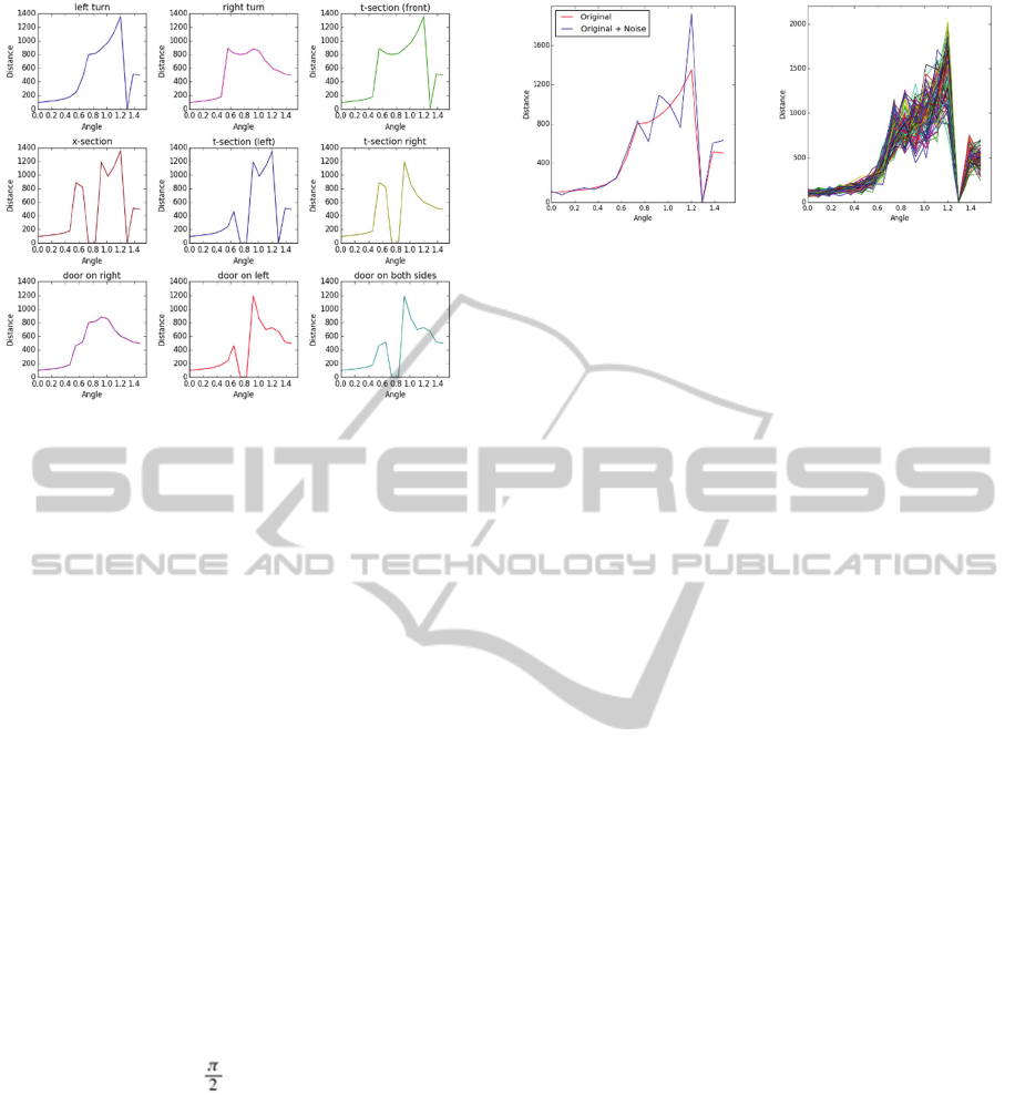
Figure 3: AIDer Laser Laser Scan Data for 9 cues.
Progressive scan angles in radians are shown on x axis,
while the y axis shows distance in inches.
3 DATA SETS
The laser mounted on AIDer is capable of scanning
180° with a granularity yielding 512 measurements
per scan. To explore machine learning techniques for
AIDer cue identification, we set aside the large data
set that would be inconvenient for explorations, and
instead we engineered a smaller data set for a
miniaturized virtual model that otherwise preserved
the geometry of the office environment. We are
returning to the larger data set at the end of the paper
when we validate our best performing technique on
that realistic set.
For the experiments, we created by hand data for
9 cues: lt (left turn), rt (right turn), ts (t-section/front),
xs (x-section), tl (left t-section), tr (right t-section), dr
(door on right), dl (door on left), and d2 (door on both
sides). In this miniaturized model every scan is a
sequence of distance measurements made with a laser
angle progressing in 17 (rather than the original 512)
steps in the interval [0, ]. The curves for all cues are
shown in Figure 3.
A visual inspection of the graphs gives hope that
the curves indeed can be correctly classified within
some noise limits. These limits can be established to
some degree by introducing elements of possible
noise that can be modeled by modifying each data
point using the normal distribution with a certain
standard deviation. That noise accounts for the
inaccuracy of the laser measurements. For example,
the type of the material from which walls are built
impacts the reading.
Figure 4: Left turn curve adjusted for distance from the cue,
and then with a noise added. Progressive scan angles in
radians are shown on x axis, while the y axis shows distance
in inches.
For illustration of the impact of distortion on the ideal
curves, the left graph in Figure 4 show the curve for
the lt (left turn) cue with overlaid sample noisy curve:
one distorted curve on the left, and with added noise.
For actual training, we generated a large number of
noisy curves. To illustrate the complexity that the
training algorithm must overcome, the right side of
Figure 4 shows a bundle of 100 curves generated for
left turn with a standard deviation of ߪ = 0.2. We used
numerous levels of noise in the experiments and
larger sample sets.
4 FEATURE VECTORS
Each of the generated noisy curves is used as a
training sample for building a clustering model. To
create a corresponding feature vector, each curve was
preprocessed. First, we normalized the data to the [-
.5, 0.5] interval, and then we applied principal
component analysis (PCA) with a hope to eliminate
redundant data dimensions, but also to visualize data
clustering (in 3 rather than 17 dimensions, so not all
nuances in the data are captured in the plot). We also
tried linear discriminant analysis (LDA), but we got
better clustering with PCA. That was important in our
case, since a visual inspection shows that certain parts
of the original ideal curves are repeated in every
pattern. We could just cut off these dimensions from
the data altogether, but instead we left it to the PCA
that formalizes such observations while also catching
similarities that are not easily visible with a naked
eye. Additionally, while the ideal data may be aligned
in some dimensions, noisy data coming from the
scanner may not be so inclined, so it’s better to let the
PCA make such decisions.
Figure 5 shows how the data is clustered using just
the first three principal components of the
preprocessed data. The 3D scatter graphs for curves
with low distortion clearly indicate that the data are
ExploringMachineLearningTechniquesforIdentificationofCuesforRobotNavigationwithaLIDARScanner
647
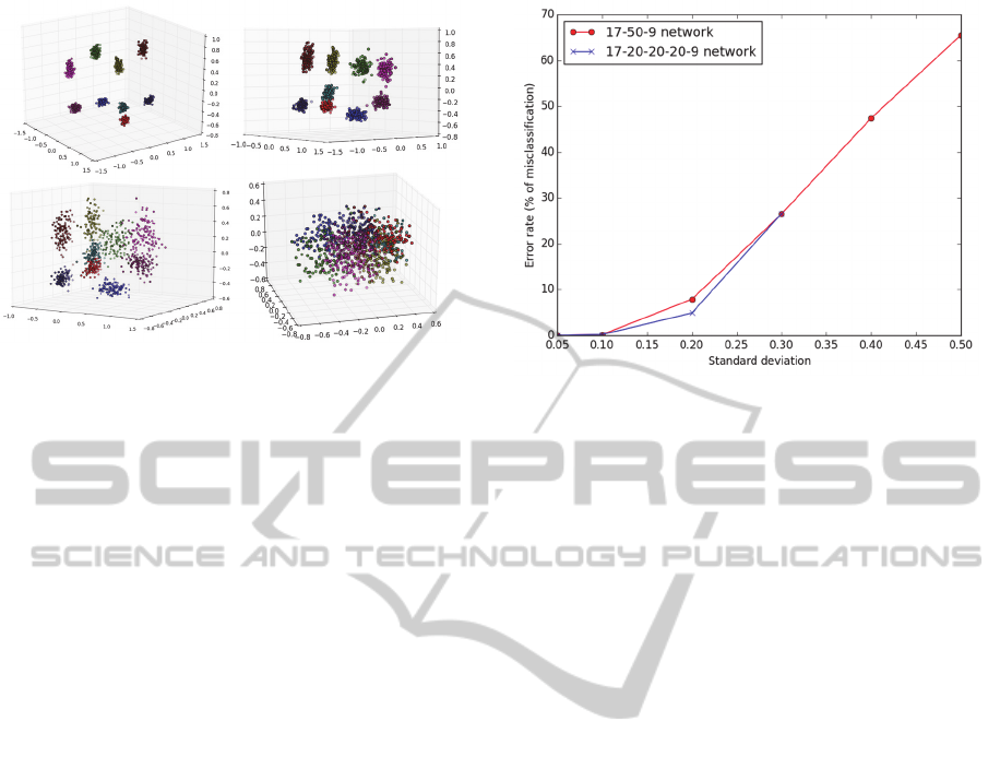
Figure 5: Visible nine clusters of feature vectors
corresponding to the nine target cues. Standard deviation of
ߪ = 0.05, ߪ = 0.1, ߪ = 0.2, and ߪ = 0.5 were used to generate
the curves (starting with the left upper corner). Please note
that the visuals are rotated to show the best perspective of
the clusters.
clustered in nine locations corresponding to the nine
target cues. The figure also illustrates the challenge in
data separation when the standard deviation is
increased. After numerous experiments, we actually
found that for best results (i.e., for the lowest error
rate) we needed to keep almost all principal
components banning one or two least significant.
Since dropping so few had minimal impact on the
efficiency of training, we ended up with using PCA
for improving odds for clustering rather than for
dimension reduction.
5 EXPLORING NEURAL
NETWORK-BASED CUE
IDENTIFICATION
With so-generated one thousands of feature vectors at
hand, we used the backpropagation neural network to
build a classifier. We also attempted to process larger
numbers (namely ten thousand), but that was taking
too much time (in excess of 12 hours on a fast iMac
running Python 3.4 and Neurolab 3.5). We tried a
number of training strategies available as options in
Neurolab, but we were consistently successful only
with the one based on the Broyden-Fletcher-
Goldfarb-Shannon (BFGS) optimization. Other
optimization methods (such gradient decent) took
much longer time, often failed to converge, and
lacked consistency in repeated attempts (i.e., they
were very dependable on the starting conditions). A
backpropagation network with BFGS optimization-
based training was converging successfully under a
Figure 6: Convergence rate of a back propagation network
with BFGS training in training with random curves
distorted with varied standard deviation.
variety of conditions and had a high rate of
identification accuracy (unless the data set was very
large as will be explained later).
Just for completeness and clarity of the setup for
the experiments, let us clearly state that we used a 17-
unit input layer (since we have 17-dimension feature
vectors), and a 9-unit binary output layer (as we have
9 cues - classification targets). We also tried a
network with one single multivariate output unit, but
that architecture did not yield a successful model.
After trying a number of network architectures,
we found that a 17-50-9 network (a single-hidden-
layer network with fifty hidden units) was performing
similarly to a 17-20-20-20-9 (three-hidden-unit
network with twenty units in each hidden layer); as
shown in Figure 6. With higher level of distortion
(standard deviation ߪ >= 0.4), the 17-20-20-20-9
network failed to train in a reasonable time. The
convergence speed was similar for both networks as
shown in Figure 7 for standard deviation ߪ = 0.1. The
figure shows the convergence rate of the networks for
one thousand randomly distorted curves generated
with two different standard deviations (with SSE used
as a measure of errors). Increasing the standard
deviation often led to increased training time (but not
always owing to the dependence on the starting
condition that are chosen automatically by the
Neurolab’s training algorithm), to a higher error rate
on the test set, and increasingly frequent failure to
converge below the target error rate. Neurolab’s
training functions detect when there is no progress
(i.e., no change in the error rate) and terminate the
training session even before hitting the limit on the
number of epochs.
The training the 17-50-9 network took
ICINCO2015-12thInternationalConferenceonInformaticsinControl,AutomationandRobotics
648

Figure 7: Comparison of convergence rates of backpropagation networks with BFGS 17-20-20-20-9 (left) and 17-50-9 (right)
with random curves distorted with standard deviation of ߪ = 0.1.
increasingly longer time for the larger ߪ, but
completed successfully. As shown in Figure 8, the
network was relatively effective in tests with the the
training set, but it became increasingly less reliable
with higher level of noise.
For testing the models, we generated another
thousand randomly distorted new curves. In tests, we
used the preprocessing transform functions
(normalization and PCA) constructed with the
training set, since the application requires that the
model is able to deal well with novelty. As it could be
expected, if the standard deviation of the test set was
the same as the one used to generate the training set,
the accuracy of the model was better than with a test
set generated with a higher standard deviation than
the one used in training.
It’s worth noting here that we did not need to use
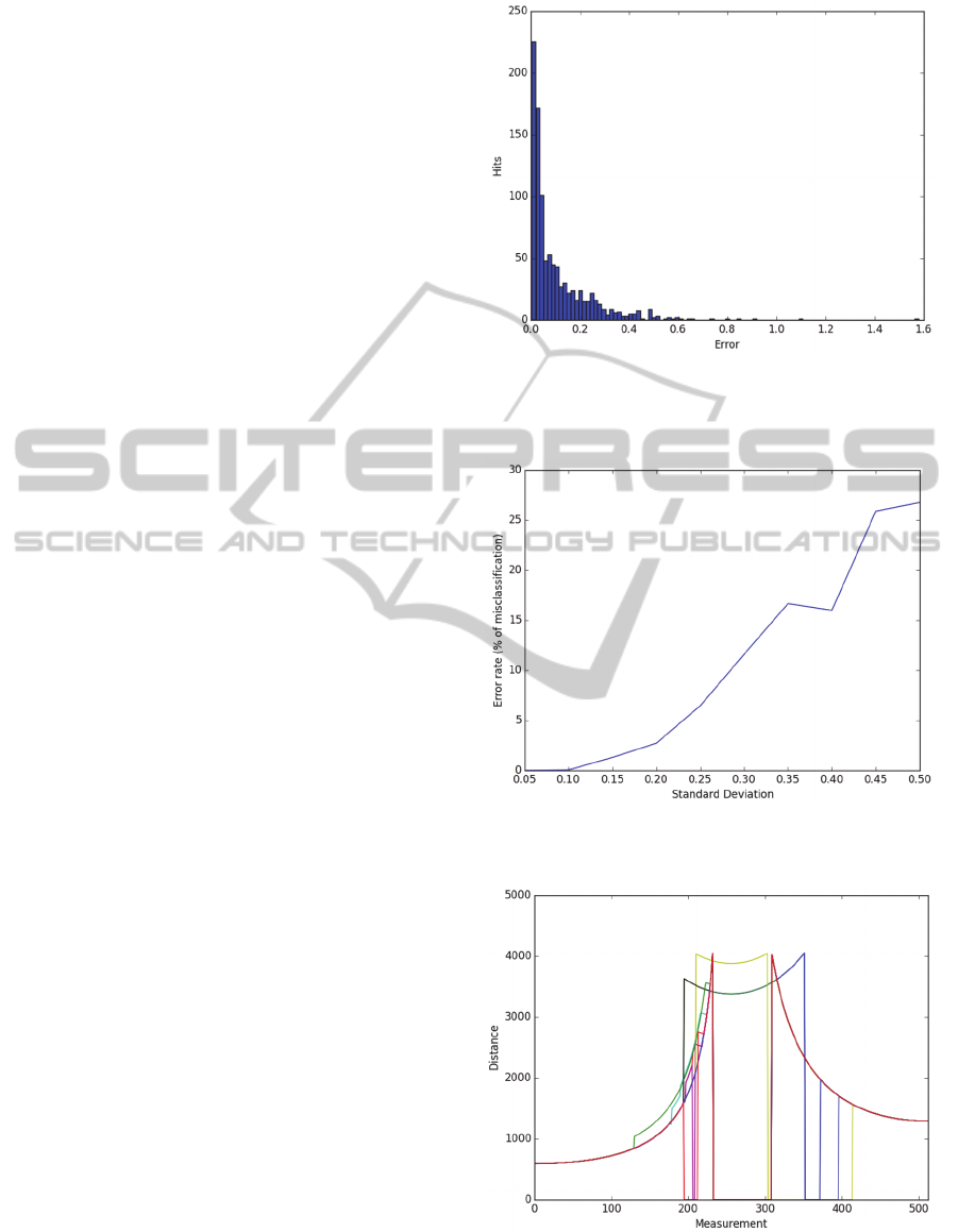
Figure 8: Performance of a 17-50-9 network expressed
through a misclassification error rate as a function of the
standard deviation used for generating curves.
Figure 9: Misclassification rate as a function of the
regularization coefficient with standard ߪ = 0.3.
any of the crossvalidation techniques as we could
generate test data at will.
6 APPLYING REGULARIZATION
To address the higher misclassification rate for higher
noise in input data, we tested several values of the
regularization coefficient to relax the clustering and
avoid overfitting. As shown in Figure 9 it was an
effective tool to improve the accuracy of
classification for noisy data.
It is interesting to note that although networks
with a non-zero regularization factor may yield higher
error rates (SSE), and even fail the training in the
traditional sense of not getting under a certain error
threshold, they can still classify correctly the data,
and therefore show lower classification error. To
ExploringMachineLearningTechniquesforIdentificationofCuesforRobotNavigationwithaLIDARScanner
649
illustrate the point, compare the rate of
misclassifications in Figure 9 with the number of
erroneous outputs made by the same network shown
in Figure 10.
It is an important distinction between applications
for classification in which the winner-takes-all
strategy is applied, and for regression; in the latter,
increased error rate would certainly be more
troublesome.
7 EXPLORING SUPPORT
VECTOR MACHINES (SVM)
FOR CUE IDENTIFICATION
We attempted to improve the performance of the
neural network models by increasing the cardinality
of the training set to ten thousands samples.
Unfortunately, as we stated earlier, the BNFS training
algorithms in the Neurolab could not deal with that
number of data points, and as a consequence failed to
converge in a reasonable time. As also previously
explained, using a reduced dimension proved to make
things worse in the experiments with a smaller
training set, so we decided to move on and try another
technique said to be very successful in classification
applications, Support Vector Machines (SVM).
We started immediately with a very large set of
training samples (ten thousands), since we were
interested in the performance of the training method
in the Scikit Learn toolkit that we used for our
explorations. Scikit Learn uses extremely efficient
scientific libraries collected under one common
umbrella of SciPy; some implemented even in Fortran
for maximal efficiency. The implementation of the
SVM in Scikt Learn has a very convenient to use API
for multi-class classification.
We preprocessed the data in the way identical to
the earlier experiments using neural networks:
MixMaxScaler and PCA. We tried to use data with
reduced dimension, but as earlier, we got better
results when keeping all dimensions.
For tests, we generated a random set of also ten
thousand data points and using the same level of
distortion (i.e., the standard deviation ߪ) as in the
training.
One immediate observation was that the SVM
training on a ten times larger data set was
dramatically faster then for the neural network using
many fewer samples. Figure 11 shows the results
from a number of experiments with a variety of
distortion levels. Comparing these results to the ones
shown in Figure 8 and 9, it is evident that in presence
Figure 10: A histogram of errors made by a model with a
regularization coefficient of 0.3 for a data set generated
with ߪ = 0.3.
Figure 11: Performance of SVM models on sets with
increasing standard deviation.
Figure 12: Ten overlaid actual 512-dimensional curves for
cue identification in actual AIDer environment. Distance is
measured in inches, and the x axis shows index of each
measurement (from 0 to 511).
ICINCO2015-12thInternationalConferenceonInformaticsinControl,AutomationandRobotics
650

of noise, the performance of the model built with
SVM exceeds by three-fold or so the capability of the
backpropagation neural network with the best
performing (with our specific data sets) BFGS
training. We used the default values of SVM
parameters from Scikit Learn.
8 CONCLUSIONS: VALIDATING
THE MODEL IN A HIGHER
DIMENSION
As we stated at the beginning of this document, the
actual scanner data has a much higher dimension: 512
rather than 17 used for our explorations of the
machine learning techniques. Figure 12 shows the
ideal cues taken from the actual physical facility (the
measurements were done by hand rather than from a
scanner; hence the adjective “ideal”). There are also
ten rather than nine cues in this data set. With the very
optimistic results from the experiments with the
SVM, we used exactly same strategy to process the
realistic data. Quite often, it’s a computational
challenge to expand the dimension of a data set thirty-
fold; it was evident in the increased processing times.
Still, the increase in the demand for time was more of
linear rather than exponential nature in spite of using
also ten thousand samples for both training and for
testing.
We need to emphasize that it was critical to
normalize the data, since some algorithms in the
Python toolkit could fail on NaNs otherwise.
Fortunately, the MinMaxScale() function from Scikit
Learn worked well, preparing data for successful
PCA as shown in Figure 13.
Subsequently, the SVM algorithms converged
nicely and performed similarly to the experiments
with the smaller data set. Figure 14 shows the results
for several levels of noise.
9 FUTURE DIRECTIONS
One of the aspects of curve shape distortion for cues
based on object boundaries is the point of view from
which the snapshot is taken. If the identification is
made quickly, then it does not matter, as the model
may be picking the level of recognition of a cue in the
ideal spot from which the training samples were
generated. Introducing such an element of distortion
with random methods is difficult, since the shape of
the cue may change more dramatically than with
application of a standard deviation, so another
approach can be to use a number of points of view
(e.g., three) and to generate snapshots of a cue taken
from these points. In this way, the training data would
include a number of views of each cue. We report on
this approach in another paper (Bieszczad, 2015).
Yet another problem omitted in this paper is the
fact that cues often are present at the same time, so
they make it to the same snapshot. We are planning
to use data sets that mix cues to some degree to test
the identification capabilities of the models trained
under such circumstances. One idea to deal with this
problem if it arises is to separate cues from curves.
Such attempts have been made by numerous
researchers, and in more complex approaches to the
localization problem (e.g., through image processing
and scene analysis).
Much harder problem to overcome is the issue of
accuracy of laser scans when dealing with various
materials from which obstacles are made and light
Figure 13: Normalized cue curves and their location in the feature space with only three most significant principal
components. The distance uses normalized values, and measurement index is shown on the x axis. The 3D plot is rotated for
best illustration of centers of the clusters.
ExploringMachineLearningTechniquesforIdentificationofCuesforRobotNavigationwithaLIDARScanner
651

conditions. These issues are of paramount importance
in outdoor navigation in an unknown terrain as
described in (Roman et al., 2007) and elsewhere.
While we plan to continue experimenting with a
robot, using a physical machine for numerous tests is
inconvenient and inefficient, so we are planning to
build a simulator with which it will be easier to test
our models.
REFERENCES
Hilde, L., 2009. Control Software for the Autonomous
Interoffice Delivery Robot. Master Thesis, Channel
Islands, California State University, Camarillo, CA.
Rodrigues, D., 2009. Autonomous Interoffice Delivery
Robot (AIDeR) Software Development of the Control
Task. Master Thesis, Channel Island, California State
University, Camarillo, CA.
Thrun, S., 1998. Learning metric-topological maps for
indoor mobile robot navigation. In Artificial
Intelligence, Vol. 99, No. 1, pp. 21-71.
Hinkel, R, and Knieriemen, T., 1988. Environment
Perception with a Laser Radar in a Fast Moving Robot.
In Robot Control 1988 (SYROCO'88): Selected Papers
from the 2nd IFAC Symposium, Karlsruhe, FRG.
Henderson, A. M., 1012. Autonomous Interoffice Delivery
Robot (AIDeR) Environmental Cue Detection. Master
Thesis, Channel Island, California State University,
Camarillo, CA.
Leonard, J., et al., 2008. A Perception-Driven Autonomous
Urban Vehicle. In Journal of Field Robotics, 1–48.
Tan, F., Yang, J., Huang, J., Jia, T., Chen, W. and Wang, J.,
2010. A Navigation System for Family Indoor Monitor
Mobile Robot. In The 2010 IEEE/RSJ International
Conference on Intelligent Robots and Systems, October
18-22, 2010, Taipei, Taiwan.
Roman, M., Miller, D., and White, Z., 2007. Roving Faster
Farther Cheaper. In 6th International Conference on
Field and Service Robotics - FSR 2007, Jul 2007,
Chamonix, France. Springer, 42, Springer Tracts in
Advanced Robotics; Field and Service Robotics.
Vilasis-Cardona, X., Luengo, S., Solsona, J., Maraschini,
A., Apicella, G. and Balsi, M., 2002. Guiding a mobile
robot with cellular neural networks. In International
Journal of Circuit Theory and Applications; 30:611–
624.
Shu, L., Xu, H., and Huang, M., 2013. High-speed and
accurate laser scan matching using classified features.
In IEEE International Symposium on Robotic and
Sensors Environments (ROSE), Page(s): 61 - 66.
Nunez, P. Vazquez-Martin, R. del Toro, J. C. Bandera, A.
and Sandoval, F., 2006. Feature extraction from laser
scan data based on curvature estimation for mobile
robotics. In IEEE International Conference Robotics
and Automation (ICRA),, pp. 1167–1172.
Zhang, L. and Ghosh, B. K., 2000. Line segment based map
building and localization using 2d laser rangefinder. In
IEEE International Conference on Robotics and
Automation (ICRA), pp. 2538–2543.
Harbl M., Abielmona, R., Naji, K.,and Petriu, E., 2010.
Neural Networks for Environmental Recognition and
Navigation of a Mobile Robot. In Proceedings of IEEE
International Instrumentation and Measurement
Technology Conference, Victoria, Vancouver Island,
Canada.
Kubota, S., Ando, Y., and Mizukawa, M., 2007. Navigation
of the Autonomous Mobile Robot Using Laser Range
Finder Based on the Non Quantity Map. In
International Conference on Control, Automation and
Systems, COEX, Seoul, Korea.
Bieszczad, A. and Pagurek, B. (1998), Neurosolver:
Neuromorphic General Problem Solver. In Information
Sciences: An International Journal 105 (1998), pp.
239-277, Elsevier North-Holland, New York, NY.
Bieszczad, A., 2015. Identifying Landmark Cues with
LIDAR Laser Scanner Data Taken from Multiple
Viewpoints. In Proceedings of International
Conference on Informatics in Control, Automation and
Robotics (ICINCO), Scitepress Digital Library.
ICINCO2015-12thInternationalConferenceonInformaticsinControl,AutomationandRobotics
652
