Fast and Robust Keypoint Detection in Unstructured 3-D Point Clouds

Jens Garstka and Gabriele Peters

Human-Computer Interaction, Faculty of Mathematics and Computer Science,

University of Hagen, D-58084 Hagen, Germany

Keywords:

3-D Keypoint Detection, 3-D Recognition, 3-D Computer Vision.

Abstract:

In robot perception, as well as in other areas of 3-D computer vision, keypoint detection is the ﬁrst major

step for an efﬁcient and accurate 3-D perception of the environment. Thus, a fast and robust algorithm for an

automatic identiﬁcation of keypoints in unstructured 3-D point clouds is essential. The presented algorithm is

designed to be highly parallelizable and can be implemented on modern GPUs for fast execution. The com-

putation is based on a convolution of a voxel based representation of the point cloud and a voxelized integral

volume. The generation of the voxel-based representation neither requires additional surface information or

normals nor needs to approximate them. The proposed approach is robust against noise up to the mean distance

between the 3-D points. In addition, the algorithm provides moderate scale invariance, i. e., it can approximate

keypoints for lower resolution versions of the input point cloud. This is particularly useful, if keypoints are

supposed to be used with any local 3-D point cloud descriptor to recognize or classify point clouds at different

scales. We evaluate our approach in a direct comparison with state-of-the-art keypoint detection algorithms in

terms of repeatability and computation time.

1 INTRODUCTION

3-D object recognition and classiﬁcation is a funda-

mental part of computer vision research. Many of the

existing recognition systems use local feature based

methods as they are more robust to occlusion and clut-

ter. In those systems keypoint detection should be the

ﬁrst major step to get distinctive local areas for dis-

criminative local feature descriptions. But a recent

survey on feature based 3-D object recognition sys-

tems (Guo et al., 2014) shows, that many major sys-

tems for local feature based 3-D object recognition

use sparse sampling or mesh decimation methods to

create a set of points on which the feature descriptors

will be computed. In terms of repeatability and in-

formativeness these methods do not result in qualiﬁed

3-D keypoints.

There are a variety of reasons why existing 3-D

keypoint detection algorithms are not used: Some of

them are sensitive to noise and some are time consum-

ing. Furthermore, there is only a handful of meth-

ods, that work with unstructured 3-D point clouds

without a time consuming approximation of local sur-

face patches or normal vectors (Pauly et al., 2003;

Matei et al., 2006; Flint et al., 2007; Unnikrishnan

and Hebert, 2008; Zhong, 2009; Mian et al., 2010).

This paper addresses the problems described

above. The proposed method is a fast and robust algo-

rithm for automatic identiﬁcation of 3-D keypoints in

unstructured 3-D point clouds. We create a ﬁlled and

watertight voxel representation (in terms of a dense

voxel connectivity) of a point cloud. This voxel rep-

resentation is convolved with a spherical convolution

kernel. The sphere works as an integral operator on all

voxels containing points of the point cloud. The con-

volution gives the proportion of voxels of the sphere

which are inside the point cloud. The proportion val-

ues are used to identify regions of interest, and from

these robust keypoints are extracted. All parts of

the algorithm are highly parallelized and thus will be

computed very quickly. The size of the convolution

kernel can be adopted to the size of the area which is

used by the local feature descriptor. Furthermore, we

can easily simulate a lower resolution point cloud by

increasing the voxel size. Therefore, we can create

keypoints for multiple resolutions. Finally we will

show, that our approach provides robust keypoints,

even if we add noise to the point cloud.

2 RELATED WORK

There are many 3-D keypoint detection algorithms

131

Garstka J. and Peters G..

Fast and Robust Keypoint Detection in Unstructured 3-D Point Clouds.

DOI: 10.5220/0005569501310140

In Proceedings of the 12th International Conference on Informatics in Control, Automation and Robotics (ICINCO-2015), pages 131-140

ISBN: 978-989-758-123-6

 2015 SCITEPRESS (Science and Technology Publications, Lda.)

that work on meshes or use surface reconstruction

methods. A brief overview is given in a recent sur-

vey paper (Guo et al., 2014). But there are only a few

of them that work directly on unstructured 3-D point

cloud data. They have been compared multiple times

(Salti et al., 2011; Dutagaci et al., 2012; Filipe and

Alexandre, 2013) and therefore, we will give just a

short overview of algorithms, which are designed to

work with point clouds only.

(Pauly et al., 2003) use a principal component

analysis to compute a covariance matrix C for the lo-

cal neighborhood of each point p. With the eigen-

values λ

, λ

and λ

they introduce the surface vari-

ation σ

(p) = λ

/(λ

+ λ

), for a neighborhood

of size n, i. e., the n nearest neighbors to p. Within a

smoothed map of surface variations Pauly et al. do a

local maxima search to ﬁnd the keypoints. A major

drawback of this method is, that the surface variation

is sensitive to noise (Guo et al., 2014).

(Matei et al., 2006) use a similar approach as

Pauly et al., but they use only the smallest eigenvalue

of the covariance matrix C for a local neighbor-

hood of a point p to determine the surface variation.

But in contrast to Pauly et al., the method from Matei

et al. provides only a ﬁxed-scale keypoint detection.

The algorithm presented by (Flint et al., 2007) is

a 3-D extension of 2-D algorithms like SIFT (Lowe,

2004) and SURF (Bay et al., 2006) called THRIFT.

They divide the spatial space by a uniform voxel grid

and calculate a normalized quantity D for each voxel.

To construct a density scale-space Flint et al. convolve

D with a series of 3-D Gaussian kernels g(σ). This

gives rise to a scale-space S(p,σ) = (D ⊗g(σ))(p)

for each 3-D point p. Finally, they compute the de-

terminant of Hessian matrix at each point of the scale

space. Within the resulting 3 ×3 ×3 ×3 matrix, a

non maximal suppression reduces the entries to local

maxima, which become interest points.

(Unnikrishnan and Hebert, 2008) introduce a 3-D

keypoint detection algorithm based on an integral op-

erator for point clouds, which captures surface vari-

ations. The surface variations are determined by an

exponential damped displacement of the points along

the normal vectors weighted by the mean curvature.

The difference between the original points and the

displaced points are the surface variations which will

be used to extract the 3-D keypoints, i. e., if a dis-

placement is an extremum within the geodesic neigh-

borhood the corresponding 3-D point is used as key-

point.

(Zhong, 2009) propose another surface variation

method. In their work they use the ratio of two succes-

sive eigenvalues to discard keypoint candidates. This

is done, because two of the eigenvalues can become

equal and thus ambiguous, when the corresponding

local part of the point cloud is symmetric. Apart from

this, they use the smallest eigenvalue to extract 3-D

keypoints, as proposed by Matei et al.

Finally, also (Mian et al., 2010) propose a surface

variation method. For each point p they rotate the lo-

cal point cloud neighborhood in order to align its nor-

mal vector n

to the z-axis. To calculate the surface

variation they apply a principal component analysis to

the oriented point cloud and use the ratio between the

ﬁrst two principal axes of the local surface as measure

to extract the 3-D keypoints.

3 OUR ALGORITHM

The basic concept of our algorithms is adopted from

a keypoint detection algorithm for 3-D surfaces in-

troduced by (Gelfand et al., 2005). To be able to

use an integral volume to calculate the inner part of

a sphere without structural information of the point

cloud, we designed a volumetric convolution of a wa-

tertight voxel representation of the point cloud and a

spherical convolution kernel. This convolution calcu-

lates the ratio between inner and outer voxels for all

voxels that contain at least one point of the 3-D point

cloud. The convolution values of the point cloud get

ﬁlled into a histogram. Keypoint candidates are 3-D

points with rare values, i. e., points corresponding to

histogram bins with a low level of ﬁlling. We clus-

ter these candidates, ﬁnd the nearest neighbor of the

centroid for each cluster, and use these points as 3-D

keypoints.

Thus, our method for getting stable keypoints in

an unstructured 3-D point cloud primarily consists of

the following steps:

1. Estimate the point cloud resolution to get an ap-

propriate size for the voxel grid.

2. Transfer the point cloud to a watertight voxel rep-

resentation and ﬁll all voxels inside of this water-

tight voxel model with values of 1.

3. Calculate a convolution with a voxel representa-

tion of a spherical convolution kernel.

4. For each 3-D point ﬁll the convolution results of

its corresponding voxel into a histogram.

5. Cluster 3-D points with rare values, i. e., 3-D

points of less ﬁlled histogram bins, and use the

centroid of each cluster to get the nearest 3-D

point as stable keypoint.

The details of these steps are provided in the sections

below.

ICINCO2015-12thInternationalConferenceonInformaticsinControl,AutomationandRobotics

132

3.1 Point Cloud Resolution

A common way to calculate a point cloud resolution

is to calculate the mean distance between each point

and its nearest neighbor. Since we use the point cloud

resolution to get an appropriate size for the voxel

grid (which is to be made watertight in the following

steps), we are looking for a voxel size which leads to

a voxel representation of the point cloud, where only

a few voxels corresponding to the surface of the ob-

ject remain empty, while as much as possible of the

structural information is preserved.

To get appropriate approximations of point cloud

resolutions, we carried out an experiment on datasets

obtained from ’The Stanford 3-D Scanning Reposi-

tory’ (Stanford, 2014). We examined the mean Eu-

clidean distances between n nearest neighbors of m

randomly selected 3-D points, with n ∈ [2,10] and

m ∈ [1,100]. The relative difference between the

number of voxels based on the 3-D points to the num-

ber of voxels based on the triangle mesh were ﬁlled

into a separate histogram for each value of n. The his-

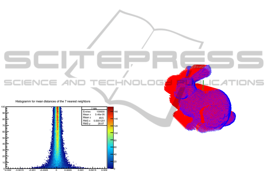
togram of the ’Stanford Bunny’ shown in ﬁgure 1 is

illustrative for all results.

Figure 1: The quality of the voxel grid based on the point

cloud resolution calculated by the mean of n = 7 nearest

neighbors. The x-axis shows the relative difference between

the number of voxels based on the 3-D points to the number

of voxels based on the triangle mesh of ’Stanford Bunny’.

The y-axis shows the number of randomly selected points

which have been used to calculate the values.

With n = 7 the absolute mean of the relative dif-

ference is at a minimum. Thus, the experiments us-

ing different 3-D objects show that an approximated

point cloud resolution with the use of 7 nearest neigh-

bors and with a sample size of 50 randomly selected

points is a good choice to get a densely ﬁlled initial

voxel grid within a small computation time.

3.2 Fast Creation of a Watertight

3-D Model

Initially we create a voxel grid of cubic voxels with

an edge length of the point cloud resolution as de-

scribed above. Each voxel containing a 3-D point is

initialized with a value of 1.0. This creates an approx-

imated voxel representation of the surface. The voxels

representing the point cloud are deﬁned as watertight,

if the voxels result in a densely connected structure

without gaps.

To be able to ﬁll inner values of objects, we as-

sume that it is known whether the point cloud repre-

sents a closed model or a depth scan, which has its

depth direction along the z-axis.

In case of a depth scan, which is very common

in robotics, we take the maximum depth value z

max

and the radius of the convolution kernel r

conv

, and set

the value of all voxels along the z-axis beginning with

the ﬁrst voxel with a value of 1 (a surface voxel) and

ending with depth of at least z

max

+ r

conv

to a value of

1, too. An illustration of this can be seen in ﬁgure 2.

Figure 2: This is a voxel representation of a view dependent

patch (depth scan) from the ’Bunny’. Blue dots represent

voxels corresponding to 3-D points. Red dots represent the

ﬁlled voxels below the surface.

In case we assume a closed model we have to ﬁll

all inner voxels. Due to variations in density of the

point cloud and the desire to keep the voxel size as

small as possible, it often occurs that the voxel surface

is not watertight. For ﬁrst tests we implemented two

different approaches to close holes in the voxel grid.

The ﬁrst implementation was based on the method

from (Adamson and Alexa, 2003). Their approach

is in fact intended to enable a ray tracing of a point

cloud. They use spheres around all points of the point

cloud to dilate the points to a closed surface. Shooting

rays through this surface can be used to close holes.

The second implementation was based on a method

by (Hornung and Kobbelt, 2006). Their method cre-

ates a watertight model with a combination of adap-

tive voxel scales and local triangulations. Both meth-

ods create watertight models without normal estima-

tion. But the major drawback of both methods con-

sists in their long computation times.

Since the method we propose should be fast, these

FastandRobustKeypointDetectioninUnstructured3-DPointClouds

133

concepts were discarded for our approach. Instead we

use a straightforward solution, which appears to be

sufﬁcient for good but fast results. The ﬁlling of the

voxel grid is described exemplary for the one direc-

tion. The calculation of the other directions is per-

formed analogously.

Let u, v and w the indexes of the 3-D voxel grid in

each dimension. For each pair (u,v) we iterate along

all voxels in w-direction. Beginning with the ﬁrst oc-

currence of a surface voxel (with a value of 1) we

mark all inner voxels by adding −1 to the subsequent

voxels until we reach the next surface voxel. These

steps are repeated until we reach the w boundary of

the voxel grid. If we added a value of −1 to the last

voxel, we must have passed a surface through a hole.

In this case we need to reset all values for (u, v) back

to the previous values.

After we did this for each dimension, all voxels

with a value ≤ −2, i. e., all voxel which have been

marked as inner voxels by passes for at least two di-

mensions, will be treated as inner voxels and their

value will be set to a value of 1. All other voxels will

get a value of 0.

We already mentioned, that, if we pass the surface

through a hole, we set back all voxel values to previ-

ous values. This might result in tubes with a width of

one voxel (see ﬁgure 3(a)). Because of that, we ﬁll

these tubes iteratively in a post-processing step, with

the following rule:

If a voxel at position (u,v,w) has a value of 0 and

at least each of the 26 neighbor voxels except of one

of the six direct neighbors (u ±1 or v ±1 or w ±1)

has a value of 0, the voxel at (u,v, w) gets a value of

1, too. The result is shown in ﬁgure 3(b).

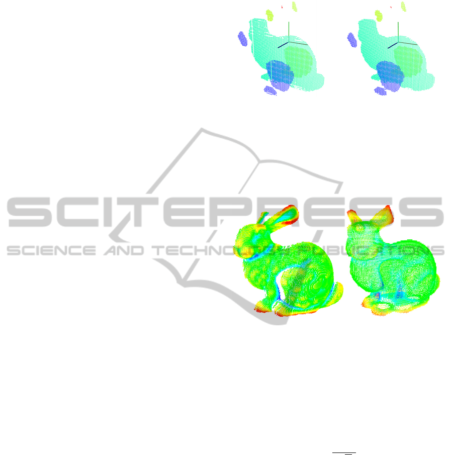
3.3 Convolution

The convolution is done with a voxelized sphere of

radius r

conv

. For a fast GPU based implementation

we use the NVIDIA FFT-implementation cuFFT. Fig-

ure 4(a) and ﬁgure 4(b) visualize the results showing

those voxels which contain 3-D points from the ini-

tial point cloud. The convolution values are in [0,1].

While values near 0 are depicted red, values near 1

are depicted blue to purple, and values of about 0.5

are depicted green.

3.4 Histograms

Following the computation of the convolution, we

have to identify all convolution values which are in-

teresting, i. e., which are less frequent. To ﬁnd those

regions of values which are less frequent, we ﬁll the

convolution values into a histogram. To get an appro-

(a) (b)

Figure 3: This ﬁgures shows sliced versions of the ﬁlled

voxel grid of the ’Bunny’. All inner voxels get ﬁlled after

the surface is passed. This is done for each direction u, v and

w. If the surface gets missed through a hole, it might lead

to tubes with a width of one voxel as shown in subﬁgure

(a). If we post-process this voxel grid, we can identify and

ﬁll those tubes. This leads to a nearly complete ﬁlled voxel

grid as shown in subﬁgure (b).

(a) (b)

Figure 4: The two subﬁgures show colored convolution re-

sults of the ’Bunny’ in full resolution using a convolution

kernel of radius r

conv

= 10pcr (pcr = point cloud resolu-

tion). Subﬁgure (a) shows a depth scan (pcr = 0.00167)

with convolution values between 0.23 (red) and 0.79 (blue)

while subﬁgure (b) shows the closed point cloud (pcr =

0.00150) with values between 0.08 (red) and 0.83 (blue).

priate amount of bins we use Scott’s rule (Scott, 1979)

to get a bin width b:

b =

3.49σ

√

, (1)

where σ is the standard deviation of N values.

In case of a depth scan we need to take into ac-

count that the convolution values at outer margins do

not show the correct values. Thus, we ignore all val-

ues of points within an outer margin r

conv

3.5 Clustering

From the histogram we select all bins ﬁlled with val-

ues of at most 1% of all points. It turned out that this

is a good choice for an upper limit since higher values

lead to large clusters. On the other hand, a signiﬁcant

smaller limit leads to fragmented and unstable clus-

ters.

ICINCO2015-12thInternationalConferenceonInformaticsinControl,AutomationandRobotics

134

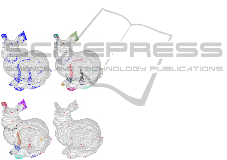
All points corresponding to the values in the se-

lected bins will be used as keypoint candidates for

clustering. Figure 5(a) shows all keypoint candidates

for the ’Bunny’. We cluster these points using the

Euclidean distance with a range limit of 3pcr. This

enables us to handle small primarily longish clusters,

e. g., the region above the bunny’s hind legs, as a sin-

gle connected cluster. Figure 5(b) illustrates the dif-

ferent clusters with separate colors.

For each cluster we calculate the centroid. Each

centroid is used to ﬁnd its nearest neighbor among the

3-D points of the corresponding cluster. This nearest

neighbor is used as 3-D keypoint. Figure 5(c) and

ﬁgure 5(d) show the results for the ’Bunny’.

(a) (b)

Figure 5: These subﬁgures illustrate the process of obtain-

ing clusters and keypoints from the set of possible can-

didates. Subﬁgure (a) shows all 3-D keypoint candidates

(blue) for the ’Bunny’. Subﬁgure (b) shows all clusters

found for an Euclidean distance with a range limit of 3pcr.

Subﬁgure (c) shows a combination of colorized clusters and

the corresponding 3-D keypoints. Finally, subﬁgure (d)

shows the isolated keypoints.

4 RESULTS

We evaluated our results with respect to the two main

quality features repeatability and computation time.

To be comparable to other approaches we used the

same method of comparing different keypoint detec-

tion algorithms and the same dataset as described by

(Filipe and Alexandre, 2013), i.e., we used the large-

scale hierarchical multi-view RGB-D object dataset

from Lai et al. (Lai et al., 2011a). The dataset con-

tains over 200000 point clouds from 300 distinct ob-

jects. The point clouds have been collected using a

turntable and an RGB-D camera. More details can be

found in another article by (Lai et al., 2011b).

4.1 Repeatability under Rotation

(Filipe and Alexandre, 2013) use two different mea-

sures to compare the repeatability: the relative and

absolute repeatability. The relative repeatability is the

proportion of keypoints determined from the rotated

point cloud, that fall into a neighborhood of a key-

point of the reference point cloud. The absolute re-

peatability is the absolute number of keypoints deter-

mined in the same manner as the relative repeatability.

To compute the relative and absolute repeatabil-

ity, we randomly selected ﬁve object classes (’cap’,

’greens’, ’kleenex’, ’scissor’, and ’stapler’) and

picked 10 point clouds within each object class ran-

domly as well. Additionally, these 50 base point

clouds were rotated around random axes at angles of

◦

, 15

◦

, 25

◦

, and 35

◦

. Afterwards, we applied our al-

gorithm on each of these 250 point clouds. For neigh-

borhood sizes n from 0.00 to 0.02 in steps of 0.001

the keypoints of the rotated point clouds were com-

pared with the keypoints of the base point clouds. If a

keypoint of a rotated point cloud fell within a neigh-

borhood n of a keypoint of the base point cloud, the

keypoint was counted. Finally, the absolute repeata-

bility was determined based on these counts for each

n as an average of the 50 corresponding point clouds

for each angle. The relative repeatability rates are the

relations between the absolute repeatabilities of the

rotated point clouds and the number of keypoints of

the base point clouds.

Figure 6 opposes relative repeatability rates of our

approach (left hand side) to the corresponding results

of four state-of-the-art keypoint detection algorithms

(right hand side). Figure 7 does the same for ab-

solute repeatability rates. The approaches evaluated

by (Filipe and Alexandre, 2013) are Harris3D (Sipi-

ran and Bustos, 2011), SIFT3D (Flint et al., 2007),

ISS3D (Zhong, 2009), and SUSAN (Smith and Brady,

1997) extended to 3-D by (Filipe and Alexandre,

2013).

In more detail, the graphs on the left of both ﬁg-

ures 6 and 7 show the average relative, resp. abso-

lute, repeatability of keypoints computed with our al-

gorithm for 5 randomly selected objects over 10 itera-

tions, i. e., with 10 different rotation axes. The graphs

FastandRobustKeypointDetectioninUnstructured3-DPointClouds

135

(a) Relative repeatability of keypoints at a rotation angle of 5

◦

(b) Relative repeatability of keypoints at a rotation angle of 15

◦

(d) Relative repeatability of keypoints at a rotation angle of 35

◦

Figure 6: Relative repeatability. Left: Our approach. Right: Four state-of-the-art approaches, diagrams taken from the

evaluation done by (Filipe and Alexandre, 2013).

ICINCO2015-12thInternationalConferenceonInformaticsinControl,AutomationandRobotics

136

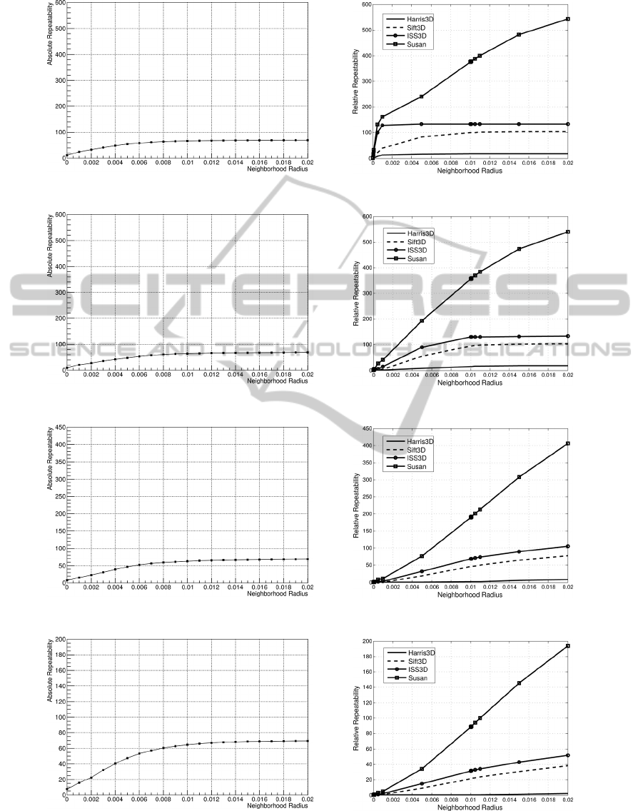
(a) Absolute repeatability of keypoints at a rotation angle of 5

◦

(b) Absolute repeatability of keypoints at a rotation angle of 15

◦

(d) Absolute repeatability of keypoints at a rotation angle of 35

◦

Figure 7: Absolute repeatability. Left: Our approach. Right: Four state-of-the-art approaches, diagrams taken from the

evaluation done by (Filipe and Alexandre, 2013). Note: The diagrams taken from Filipe and Alexandre have wrong axis

labels. However, they contain the absolute repeatability of keypoints.

FastandRobustKeypointDetectioninUnstructured3-DPointClouds

137

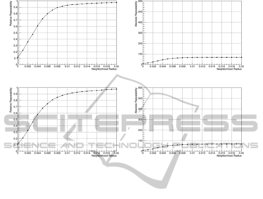
(a) Repeatability for a point cloud with 0.5pcr additional random noise at a rotation angle of 5

◦

(b) Repeatability for a point cloud with 0.5pcr additional random noise at a rotation angle of 15

◦

Figure 8: Our approach with additional noise. Left: Relative repeatability. Right: Absolute repeatability.

on the right of both ﬁgures are taken from the evalua-

tion done by (Filipe and Alexandre, 2013).

It is striking, that the relative repeatability rates

of our approach are considerably higher for large ro-

tation angles than those of all other state-of-the-art

approaches that have been compared by Filipe and

Alexandre. Only for an rotation angle of 5

◦

one of

the other algorithms (ISS3D) is able to outperform

our approach signiﬁcantly in the range of small neigh-

borhood radii. On the other hand, the results of our

algorithm in terms of absolute repeatability of key-

points are in general less convincing, although for all

of the condsidered rotation angles it outperforms one

of the other approaches (Harris3D). For a rotation an-

gle of 35

◦

our algorithm outperformes even three of

the other approaches considered (Harris3D, SIFT3D,

and ISS3D).

4.2 Repeatability under Noise

Furthermore, we have repeated the described simula-

tions for point clouds with additional random noise

at a level of 0.5 times of the point cloud resolution.

The graphs of ﬁgure 8 display the average repeatabil-

ity rates (relative and absolute) for point clouds with

added noise. The differences between these curves

and their corresponding curves from the simulations

without noise are negligible, which shows that our ap-

proach is able to cope with a fair amount of noise, as

well.

4.3 Computation Time

To calculate average computation times we computed

the 3-D keypoints 10 times for each point cloud. The

system conﬁguration we used for all experiments is

given in table 1. The computation time of our al-

gorithm correlates with the number of voxels, i. e.,

with the dimensions of the voxel grids, which must be

powers of two. Measured average computation times

in dependence of voxel grid dimensions are given in

table 2.

The computation time for most of the point clouds

was below 1s. For many of the point clouds the com-

putation time fell within a range below 300ms. The

average computation time for all 250 point clouds

which were used to compare the repeatability rates

was 457ms. This is considerably fast, especially in

comparison to the average computation times of Har-

ris3D (1010ms) and ISS3D (1197ms), which have

been determined on the same system.

ICINCO2015-12thInternationalConferenceonInformaticsinControl,AutomationandRobotics

138

Table 1: System conﬁguration for experiments.

System conﬁguration

Processor: Intel Xeon E5630 @2.53GHz

Memory: 12 GB

GPU: NVIDIA GeForce GTX 670

GPU memory: 2 GB GDDR5

OS: Debian GNU/Linux

NVIDIA driver: 340.32

Table 2: Average computation times.

Voxel Grid Dimension Time

512 ×256 ×128 ≈ 1500ms

256 ×256 ×128 ≈ 700ms

256 ×256 ×64 ≈ 300ms

256 ×128 ×128 ≈ 350ms

256 ×128 ×64 ≈ 180ms

128 ×128 ×128 ≈ 200ms

128 ×128 ×64 ≈ 110ms

128 ×64 ×64 ≈ 60ms

64 ×64 ×64 ≈ 35ms

5 CONCLUSION

In this paper we have presented a fast and robust ap-

proach for extracting keypoints from an unstructured

3-D point cloud. The algorithm is highly paralleliz-

able and can be implemented on modern GPUs.

We have analyzed the performance of our ap-

proach in comparison to four state-of-the-art 3-D key-

point detection algorithms by comparing their results

on a number of 3-D objects from a large-scale hierar-

chical multi-view RGB-D object dataset.

Our approach has been proven to outperform other

3-D keypoint detection algorithms in terms of relative

repeatability of keypoints. Results in terms of abso-

lute repeatability rates are less signiﬁcant. An impor-

tant advantage of our approach is its speed. We are

able to compute the 3-D keypoints within a time of

300ms for most of the tested objects.

Furthermore, the results show a stable behavior of

the keypoint detection algorithm even on point clouds

with added noise. Thus, our algorithm might be a

fast and more robust alternative for systems that use

sparse sampling or mesh decimation methods to cre-

ate a set of 3-D keypoints.

REFERENCES

Adamson, A. and Alexa, M. (2003). Ray tracing point

set surfaces. In Shape Modeling International, 2003,

pages 272–279. IEEE.

Bay, H., Tuytelaars, T., and Van Gool, L. (2006). Surf:

Speeded up robust features. In Computer Vision–

ECCV 2006, pages 404–417. Springer.

Dutagaci, H., Cheung, C. P., and Godil, A. (2012). Eval-

uation of 3d interest point detection techniques via

human-generated ground truth. The Visual Computer,

28(9):901–917.

Filipe, S. and Alexandre, L. A. (2013). A comparative eval-

uation of 3d keypoint detectors. In 9th Conference on

Telecommunications, Conftele 2013, pages 145–148,

Castelo Branco, Portugal.

Flint, A., Dick, A., and Hengel, A. v. d. (2007). Thrift: Lo-

cal 3d structure recognition. In Digital Image Comput-

ing Techniques and Applications, 9th Biennial Confer-

ence of the Australian Pattern Recognition Society on,

pages 182–188. IEEE.

Gelfand, N., Mitra, N. J., Guibas, L. J., and Pottmann, H.

(2005). Robust global registration. In Symposium on

geometry processing, volume 2, page 5.

Guo, Y., Bennamoun, M., Sohel, F., Lu, M., and Wan,

J. (2014). 3d object recognition in cluttered scenes

with local surface features: A survey. IEEE Trans-

actions on Pattern Analysis and Machine Intelligence,

99(PrePrints):1.

Hornung, A. and Kobbelt, L. (2006). Robust reconstruction

of watertight 3d models from non-uniformly sampled

point clouds without normal information. In Proceed-

ings of the Fourth Eurographics Symposium on Geom-

etry Processing, SGP ’06, pages 41–50, Aire-la-Ville,

Switzerland, Switzerland. Eurographics Association.

Lai, K., Bo, L., Ren, X., and Fox, D. (2011a). A large-

scale hierarchical multi-view rgb-d object dataset. In

Robotics and Automation (ICRA), 2011 IEEE Interna-

tional Conference on, pages 1817–1824. IEEE.

Lai, K., Bo, L., Ren, X., and Fox, D. (2011b). A scalable

tree-based approach for joint object and pose recogni-

tion. In AAAI.

Lowe, D. G. (2004). Distinctive image features from scale-

invariant keypoints. International Journal of Com-

puter Vision, 60:91–110.

Matei, B., Shan, Y., Sawhney, H. S., Tan, Y., Kumar, R., Hu-

ber, D., and Hebert, M. (2006). Rapid object indexing

using locality sensitive hashing and joint 3d-signature

space estimation. Pattern Analysis and Machine Intel-

ligence, IEEE Transactions on, 28(7):1111–1126.

Mian, A., Bennamoun, M., and Owens, R. (2010). On the

repeatability and quality of keypoints for local feature-

based 3d object retrieval from cluttered scenes. In-

ternational Journal of Computer Vision, 89(2-3):348–

361.

Pauly, M., Keiser, R., and Gross, M. (2003). Multi-scale

feature extraction on point-sampled surfaces. In Com-

puter graphics forum, volume 22, pages 281–289. Wi-

ley Online Library.

Salti, S., Tombari, F., and Stefano, L. D. (2011). A per-

formance evaluation of 3d keypoint detectors. In

3D Imaging, Modeling, Processing, Visualization and

Transmission (3DIMPVT), 2011 International Con-

ference on, pages 236–243. IEEE.

FastandRobustKeypointDetectioninUnstructured3-DPointClouds

139

Scott, D. W. (1979). On optimal and data-based histograms.

Biometrika, 66(3):pp. 605–610.

Sipiran, I. and Bustos, B. (2011). Harris 3d: a robust exten-

sion of the harris operator for interest point detection

on 3d meshes. The Visual Computer, 27(11):963–976.

Smith, S. M. and Brady, J. M. (1997). Susana new approach

to low level image processing. International journal

of computer vision, 23(1):45–78.

Stanford (2014). The stanford 3d scanning repository.

http://graphics.stanford.edu/data/3Dscanrep/.

Unnikrishnan, R. and Hebert, M. (2008). Multi-scale in-

terest regions from unorganized point clouds. In

Computer Vision and Pattern Recognition Workshops,

2008. CVPRW’08. IEEE Computer Society Confer-

ence on, pages 1–8. IEEE.

Zhong, Y. (2009). Intrinsic shape signatures: A shape de-

scriptor for 3d object recognition. In Computer Vision

Workshops (ICCV Workshops), 2009 IEEE 12th Inter-

national Conference on, pages 689–696. IEEE.

ICINCO2015-12thInternationalConferenceonInformaticsinControl,AutomationandRobotics

140