Integrating Particle Swarm Optimization with Analytical Nonlinear

Model Predictive Control for Nonlinear Hybrid Systems

Jean Thomas

FIE, Beni-Suef University, Ben-Suef, Egypt

Keywords: Hybrid Systems, Nonlinear Model Predictive Control, Particle Swarm Optimization.

Abstract: The computation load remains the main challenge facing the control techniques of hybrid systems with

discrete and continuous control signals. In this paper, a new hybrid controller based on Analytical Nonlinear

Model Predictive Control (ANMPC) and Particle Swarm Optimization (PSO) for nonlinear hybrid systems

is presented. The proposed controller offer sub-optimal solution in reasonable time while respecting the

given constraints. The new developed technique is not considered as a computation burden, thus real-time

implementation is possible for many hybrid systems. Besides, it can be applied directly to the nonlinear

models, avoiding linearization which may lead to inaccurate model and unexpected behaviour. An

application of the proposed controller to a three tanks example is presented.

1 INTRODUCTION

Many real systems can be modelled as hybrid

systems with discrete and continuous input signals.

Several control techniques have been proposed in

literature to control hybrid systems, among them

Model Predictive Control (MPC) has been

considered as one of the most effective techniques

that can control linear hybrid systems. However the

computation burden associated with the mixed

integer linear/quadratic optimization problems

remains the main challenge facing real-time

application. Several techniques and algorithms have

been proposed in literature to reduce the

computation load; for example (Thomas et al., 2003,

2004) proposed using multi-MLD models rather

than using one global Mixed Logical Dynamical

(MLD) (Bemporad and Morari, 1999) model with

bigger number of variables, in (Thomas et al., 2006)

a MPC for state partition based MLD model is

proposed to use simpler models. A techniques based

on genetic algorithm is proposed in (Olaru et al,

2004) and in (Thomas et al., 2005). Explicit-MPC is

proposed in (Bemporad et al., 2000a and 2000b)

where the optimization problem is treated as a multi-

parametric problem solved off-line; and hence on-

line computation reduces to a function evaluation.

However, all these techniques have been developed

for linear hybrid systems.

An Analytical Nonlinear Model Predictive

Control (ANMPC) technique for linear induction

motor is proposed in (Thomas and Hansson, 2010

and 2013), and ANMPC for nonlinear hybrid

systems with discrete inputs only is presented in

(Thomas, 2012). The proposed ANMPC controller

based on enumerating all possible inputs

combination and calculating analytically the cost

function and then selects the input combination

which minimizes the cost function. The author of

(Thomas, 2012) shows that ANMPC lead to MPC

with lower computation load compared to other

techniques proposed in literature i.e. standard B&B,

explicit MPC for the considered classes of hybrid

systems with discrete inputs only, and that ANMPC



an take into account state and output constraints.

This paper propose extending the ANMPC

controller by integrating it with Particle Swarm

Optimization (PSO) (Kennedy and Eberhart, 1995)

and show that the new proposed controller can be

applied effectively to nonlinear hybrid systems with

discrete and continuous inputs. This algorithm

reduces efficiently the computation load while

respecting the given input, states and output

constraints. Besides, the new proposed technique

can control directly nonlinear hybrid systems

avoiding linearization which may lead to inaccurate

model and unexpected behaviour.

The rest of the paper is organized as following;

section 2 briefly presents the concepts of MPC and

294

Thomas J..

Integrating Particle Swarm Optimization with Analytical Nonlinear Model Predictive Control for Nonlinear Hybrid Systems.

DOI: 10.5220/0005570702940301

In Proceedings of the 12th International Conference on Informatics in Control, Automation and Robotics (ICINCO-2015), pages 294-301

ISBN: 978-989-758-122-9

 2015 SCITEPRESS (Science and Technology Publications, Lda.)

PSO. The proposed ANMPC integrated with PSO

controller is developed in section 3. Application of

the proposed controller to a three-tanks example is

considered in section 4. Finally conclusion and some

remarks are given in section 5.

2 CONCEPTS OF MPC AND PSO

CONTROLLERS

2.1 Model Predictive Control

Predictive control was first developed at the end of

1970s, and was published by Richalet et al., (1978).

In the 1980s, many methods based on the same

concepts are developed. Those types of controls are

now grouped under the name Model Predictive

Control (MPC) (Camacho and Bordons, 1999). MPC

has proved to efficiently control a wide range of

applications in various industries.

The main idea of predictive control is to use a

model of the plant to predict future outputs of the

system. Based on this prediction, at each sampling

period, a sequence of future control values is

developed through an on-line optimization process,

which maximizes the tracking performance while

satisfying constraints. Only the first value of this

optimal sequence is applied to the plant. The whole

procedure is repeated again at the next sampling

period according to the ‘receding’ horizon strategy

(Maciejowski, 2002). The objective is to lessen the

future output error to zero with minimum input

effort. The cost function to be minimized is

generally a weighted sum of square predicted errors

and square future control values, e.g., in Generalized

Predictive Control (Clarke et al., 1987):

[]



−++

++−+=

jku

jkwkjkyNNJ

)1(

)()(

),(

(1)

where

uy,

are the predicted output and the control

signal respectively.

NN,

are the prediction

horizons and the control horizon, respectively.

are weighting factors. The control horizon permits a

decrease in the number of the calculated future

control assuming

0)( =+Δ jku

for

Nj ≥

)( jkw +

is the reference trajectory.

Constraints over the control signal, the outputs

and the control signal changing, can be added to the

cost function:

maxmin

)(

ykyy

ukuu

≤≤

Δ≤Δ≤Δ

≤≤

(2)

The solution of (1) gives the optimal sequence of

the control signal over the horizon

while

respecting the given constraints of (2).

A fundmental difficulty of the MPC approach is

the requirement to solve constrained nonlinear,

nonconvex optimization problems. A linearized

model of nonlinear systems is commonly used for

MPC controller. However, this lineariza-tion

introduce model mismatches which affect the

control performance, as the MPC performance

depends largely on the accuracy of the process’

model.

2.2 Particle Swarm Optimization

The particle swarm optimization (PSO) algorithm is

a population-based search algorithm inspired by the

social behavior of birds within a flock (Kennedy and

Eberhart, 1995). Particle Swarm has two primary

operators: Position and Velocity. Each particle

representing a potential solution is maintained

within a swarm. The position of each particle is

adjusted according to the experience of itself and its

neighbours. During each generation, each particle is

accelerated toward the particle’s previous best

position

, and the global best position

. At each

iteration, a new velocity value for each particle is

calculated based on its current velocity, the distance

from its previous best position, and the distance

from the global best position. The new velocity

value is then used to calculate the next position of

the particle in the search space. This process is then

reiterated a set number of times, or until a minimum

error is achieved. The PSO with Constriction

Coefficient is considered where velocity and

position are updated according to the following

equations (Clerc and Kennedy, 2002):

))]1((

))1(()1([)(

−−+

+−−+−=

txgrc

txprctvtv

ijj

iijijij



(3)

)()1()( tvtxtx

ijijij

+−=

(4)

where

)(tx

)(tv

and

are the position,

velocity and best personal position of particle

, in

dimension

nj ,,2,1 =

at iteration

, where

the dimension of the system inputs.

is the global

best position in dimension

and

are

IntegratingParticleSwarmOptimizationwithAnalyticalNonlinearModelPredictiveControlforNonlinearHybrid

Systems

295

constants, and

are random values in the

range [0;1].

is the constriction coefficient.

PSO has been found to be robust in solving

continuous nonlinear optimization problems as well

as capable of generating high quality solutions with

more stable and faster convergence characteristics,

and shorter calculation times than other stochastic

methods. It has been shown in the literature that

PSO can efficiently control wide range of systems

especially those with continuous control signals, see

for example (Sedighizadeh and Masehian, 2009),

(Poli, 2008) and references therein.

3 INTEGRATING PSO WITH

ANMPC FOR NONLINEAR

HYBRID SYSTEMS

The main ideas of the proposed controller;

integrating Particle Swarm Optimization with the

Analytical Nonlinear Model Predictive Control

(PSO-ANMPC), for nonlinear hybrid systems are:

• Using the PSO algorithm, find iteratively the

optimal/sub-optimal solution for the continuous

control signals that minimize the fitness function.

• For each solution (particle) of the continuous

control signals, find the best combination of the

discrete control signals using the ANMPC.

• The fitness function of the PSO is the

optimization cost function of the MPC controller.

Each particle’s position in the swarm integrated

with its best combination of discrete inputs, together,

represents a solution to the NMPC optimization

problem. i.e., the inclusion of the control sequence

over the control horizon. Thus, each particle

dimension is

Nn ×

, and the dimension of the

optimization vector of the ANMPC is

Nn ×

where

nn , are the number of continuous input

variables and discrete input variables respectively.

The effectiveness of each solution is calculated

through the fitness function, which in this case is the

considered cost function of the NMPC controller.

However, it is important to mention here that PSO is

a gradient-free technique, thus any cost function that

represents the desired behavior can be chosen. The

proposed technique avoids any linearization

technique for minimization, albeit at an increased

computational complexity.

The global best PSO is considered where each

particle is connected to and able to obtain

information from every other particle in the swarm.

(Bratton and Kennedy, 2007). Global best PSO

exhibits very fast convergence rates which are much

needed for predictive control application.

Considering the discrete input variables, there

are limited or finite numbers of possible input

combinations for the discrete input variables i.e.

k χu ∈)(

, where

is the set of possible

discrete input combinations. Thus the optimal

control signal for these variables will be one

combination of the possible input combinations.

The PSO-ANMPC can be implemented through

the following Algorithm:

Algorithm 1

1- Let

is a particle in the swarm for

Nk ,,2,1 =

, where

is number of

particles in the population.

[

]

)1(,),1(),(: −++== Nkkkp

cccckk

uuuu 

and let:

[

]

ddddi

Nkkk χuuuu ∈−++= )1(,),1(),( 

is the i-

possible discrete control sequence

over horizon N

Initializing the particles position and velocity

of the PSO, and let

∞=

opt

For

Nj :1=

(

max. number of iterations)

For each

while

is non empty, where

the set of possible input combinations

over horizon N

Select

χu ∈

, and remove it from

the set

Compute

J the cost function

according to the control combination

௜

, where:

[]

dci

uuu = .

opt

JJ <

opt

JJ =

, and

uu =

End

end

End

9- update the particles position and velocity

End

10-

opt

uu =

the optimal control signal

This technique which we call it PSO-ANMPC has

many advantages. It reduces the computation time

significantly; because from one hand: computing

analytically the cost function is faster than building

ICINCO2015-12thInternationalConferenceonInformaticsinControl,AutomationandRobotics

296

or reformulating the problem as MIQP or MILP

problem and then solving it, and from the other hand

the proposed analytical NMPC has often less

number of possible input combination than

formulating it classically in a hybrid system

framework, e.g. MLD systems (Bemborad and

Morari, 1999); to explain that in a simple way,

consider a system with one discrete input variable

which may have a value among

possible discrete

values, this will be modeled in the MLD form by

binary variables which leads to a number of possible

input combinations over control horizon

equal

Nm×

, while the number of possible input

combinations with the proposed PSO-ANMPC

controller for the same system will equal

m only.

One of the main advantages of the proposed

controller is its ability to deal directly with nonlinear

hybrid systems, where modeling and controlling of

nonlinear hybrid systems is normally a hard task and

it is very common to linearize the model, but this

linearization could lead to a complex system with

many different linear models around different

operating points and/or could introduces uncertainty

which may lead to inaccurate model affecting the

efficiency of designed or used controller. The

advantage of the technique presented here is that we

do not need to linearize the system, and non-linear

dynamics can be directly used to calculate the new

states and outputs. Moreover, The proposed

controller is easy to construct, to tune and to

implement.

3.1 Reduction Algorithm

To avoid examining all possible discrete input

combinations over the control horizon

the

flowing Algorithm is proposed.

Algorithm 2

1- Initializing with

0)(, =∞= kJJ

opt

For

{}

,,2,1, ∈u

where ݏ is the total

number of possible input combinations over

horizon ܰ

For

Nj :1=

Compute

)( jkJ

the cost function

according to the control combination

for horizon j as follows:

()( )

()

)1()(

−+++

+−+=+

jkjkf

jkJjkJ

where

()( )

(

)

1, −++ jkjkf

is the cost

at instant

()

jk +

due to the control signal

()

1−+ jk

opt

JjkJ >+ )(

Break and go to step 2

end

Nj =

)()( NkJJJNkJ

optopt

+=→<+

end

End

opt

JJ =

the optimal solution

Algorithm 2 stops the cost function calculations

at prediction step

()

jk + where

Nj <<1

for the

control sequence

over the horizon

if the cost

function at this prediction step is higher than the

current upper boundary

opt

Algorithm 2 could also be used as suboptimal

solution if the computation time is higher than the

sampling time, the Algorithm could stop at any

instant and send the control signals according to the

current

opt

as a suboptimal solution.

3.2 Constraints

In this section, we describe how system constraints

can be included in the optimization problem so that

PSO-ANMPC can offer a suboptimal solution while

respecting the given constraints.

3.2.1 Input Constraints

Constraints over the control signal

ukuu

maxmin

)( ≤≤

can be implemented by

limiting the search space in the PSO algorithm:

[

]

maxmin

,)(

jjij

xxtx ∈

, where

maxmin

are the

control signal constraints

maxmin

respectively, given that the discrete control signals

are limited by their discrete values.

Constraints over the control signal variation

max

)(

uku Δ≤Δ

can be represented through the

particles velocity limits, as follows:







≤

maxmax

max

)(

)()(

)(

jijj

jijij

VtvifV

Vtviftv

(5)

IntegratingParticleSwarmOptimizationwithAnalyticalNonlinearModelPredictiveControlforNonlinearHybrid

Systems

297

where

maxj

is the maximum allowable control

variation for the control element

3.2.2 Output and System States Constraints

Output signals and system states can be subject to

hard and/or soft constraints. Hard constraints could,

for example, relate to safety or physical constraints,

while soft constraints may be related to economic

constraints or better working conditions.

Both of hard and soft constraints can be included

in the proposed controller. Hard constraints on

output and state variables can be simply considered

by adding the following line to Algorithm 2:

∞=+→> )()()(

maxmax

jkJyxyxif

(6)

Thus any control combination which will lead to

violation of the output or state hard constraints will

be avoided.

Soft constraints which allow, at a prise,

temporary the violation of some constraints, can also

be included as following:

+≤ )()(

maxmax

xyxy (7)

Adding the following term to the cost function:

()()

jkQjkjkJ

+++=+ εε)(

(8)

where

are positive definite weighting matrix.

This additional term in Equation (8) penalize the

violation of soft constraints, pushing the system to

have zeros=

ε . Effectively, we are saying that the

constraints are allowed to be violated to a degree,

but doing so costs, and should thus be avoided if

possible.

4 APPLICATION

The proposed control strategy is applied on the three

tanks example. The simplified physical description

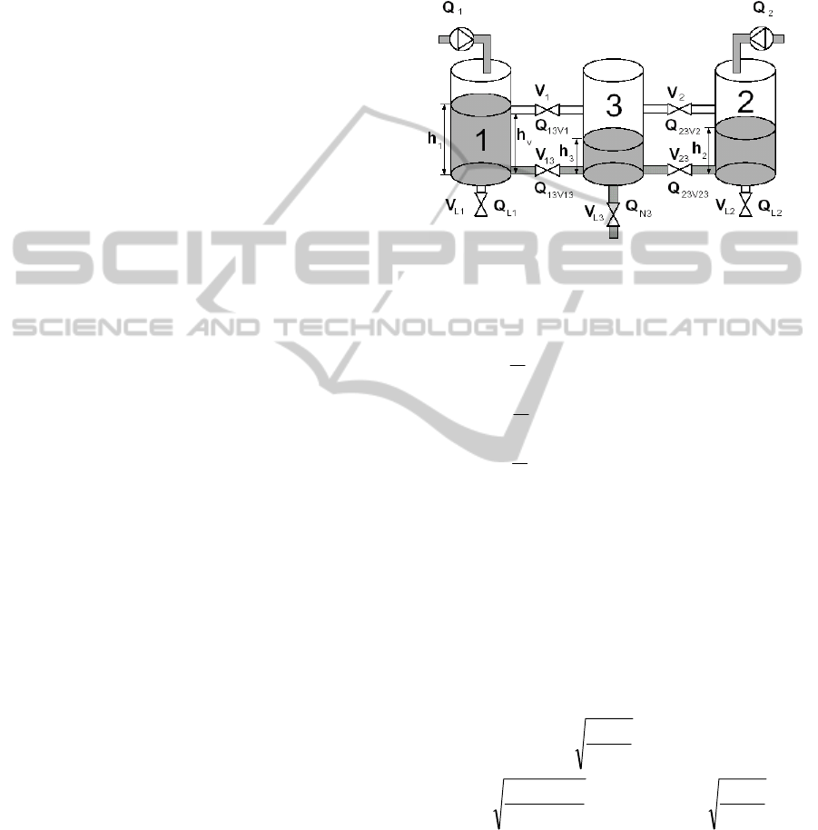
of the three tanks system is presented in Figure 1

(see Dolanc et al., 1997, for more details).

The system consists of three tanks, filled with

water by two independent pumps acting on tanks 1

and 2. These two pumps are continuously

manipulated from 0 up to a maximum flow

and

Q respectively. Four switching valves

V ,

and

V control the flow between the tanks, those

valves are assumed to be either completely opened

or closed (

lyrespective 0or 1=

). The

manual valve controls the nominal outflow of the

middle tank. It will be assumed in further

simulations that the

and

valves are always

closed and

is open. The liquid levels to be

controlled are denoted

and

for each tank

respectively.

Figure 1: COSY three tank benchmark system.

The conservation of mass in the tanks provides

the following differential equations:

)

2323

2231313113

(

)

23232232

(

)

13131131

(

−+

+++=

−−=



(9)

where the

sQ'

denote the flows and A is the

cross-sectional area of each of the tanks. The

Toricelli’s law provides the expressions of the flows

through the valves, which are given by the relations:

max

2,1,

max

:where

3333

)

,max(),(max(

)

(

Vii

−

≈

−≈

(10)

From these expressions, a model is derived with

the following variables:

23132121

[

321

[

V V V V QQ

h hh

(11)

The following specifications are considered:

starting from zero levels (the three tanks being

ICINCO2015-12thInternationalConferenceonInformaticsinControl,AutomationandRobotics

298

empty), the objective of the control strategy is to

reach the liquid levels

m 5.0

and

m 1.0

As presented in (Thomas et al., 2006), studying

the dynamic behavior of the three tanks, starting

from zero levels to the desired ones, enables to

divide the state space into three main regions, each

one with its adequate simple MLD model; for

example in the sub-region where the liquid level in

the three tanks are less than the valves level, it

clearly appears that the two valves

and

of the

input vector are not in progress, thus

231321

[ V V QQ=u

Obviously the particles of PSO will consider the

continuous signals (the two pumps), while ANMPC

will investigate the best position combination of the

four valves. The proposed PSO-ANMPC has been

implemented in simulation to reach the level

specification with the following parameters: The

parameters of the PSOMPC controller that give a

good response are:

05.2

== cc

73.0=

, with

10 particles per swarm and a maximum number of

iterations 10. A control horizon

2==

chosen. Weights in the objective function (1) have

been chosen as

)100000,1000,10000.(diag=

and

. Search space and velocity limits are chose

according to the pumps limits as follows:

[]

0001.0,

,,,

max

min

max

























−





































∈

Qwhere

The global best PSO is used for the PSO with a

constriction coefficient. The solution at instant

1−k

is memorized and introduced as a particle in the

initial population at instant

. The results are

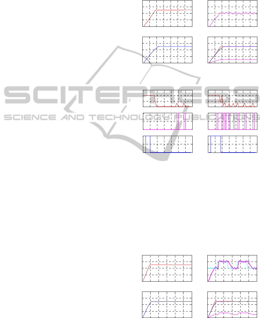
presented on Figure 2 for the tanks levels and on

Figure 3 for the control signals. The level of the

third tank oscillates around 0.1 as

1.0

does not

correspond to an equilibrium point. Consequently,

the system opens and closes the two valves

V and

to maintain the level in the third tank around the

desired level of 0.1m. The system has been

simulated in Matlab envirement.

The computation times per step is in order of ms.

i.e. is much smaller than the sampling time (the

sampling time of the three tanks benchmark is 10 s.).

Thus real-time application is possible even for

longer horizon. The PSO-ANMPC technique

reduces the computation time and provides

opportunities for real-time implementation; avoiding

exponential explosion of the algorithm.

Figure 2: Water levels in the three tanks.

Figure 3: Controlled variables.

Figures 4 and 5 respectively present the three

tanks levels and the control signals with PSO-

ANMPC technique, where the desired level in the

third tank is changing. It can be seen that the

proposed controller can successfully tracking the

desired levels. It must be noticed that the variation

of the third tank level from 0.15 to 0.1 takes more

time than the variation from 0.1 to 0.15, due to the

benchmark physical features.

Increasing the number of particles per swarm

and the maximum number of iteration will improve

Figure 4: Water levels in the three tanks –

changes.

0 5 10 15 20 25 30 35

0.2

0.4

0.6

0.8

Level h1

0 5 10 15 20 25 30 35

0.2

0.4

0.6

0.8

Sampling Instants

Levels h1, h2 and h3

0 5 10 15 20 25 30 35

0.05

0.1

0.15

0.2

Level h3

0 5 10 15 20 25 30 35

0.2

0.4

0.6

0.8

Sampling Instants

Level 2

0 5 10 15 20 25 30 35

0.5

1.5

x 10

-4

Input Q1

0 5 10 15 20 25 30 35

0.5

1.5

x 10

-4

Input Q2

0 5 10 15 20 25 30 35

0.5

0 5 10 15 20 25 30 35

0.5

0 5 10 15 20 25 30 35

0.5

Sampling Instants

V13

0 5 10 15 20 25 30 35

0.5

Sampling Instants

V23

0 10 20 30 40 50 60

0.2

0.4

0.6

0.8

Level h1

0 10 20 30 40 50 60

0.2

0.4

0.6

0.8

Sampling Instants

Levels h1 , h2 and h3

0 10 20 30 40 50 60

0.05

0.1

0.15

0.2

Level h3

0 10 20 30 40 50 60

0.2

0.4

0.6

0.8

Sampling Instants

Level h2

IntegratingParticleSwarmOptimizationwithAnalyticalNonlinearModelPredictiveControlforNonlinearHybrid

Systems

299

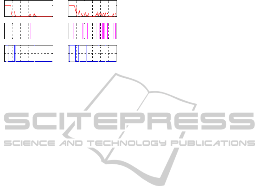
Figure 5: Controlled variables –

changes.

the suboptimal solution, and increases the

opportunities to find the optimal solution; however

this will increase the computation time. The

selection of the number of particles and the

maximum number of iteration is a trade-off, and is

based on the dynamics of the process to be

controlled.

5 CONCLUSIONS

This paper presented integrating Particle Swarm

Optimization with Analytical Nonlinear Model

Predictive Control (PSO-ANMPC) for constrained

nonlinear hybrid systems with discrete and

continuous control signals. The proposed PSO-

ANMPC controller offers a suboptimal solution in

reasonable time, thus increases the opportunities of

real-time application for many nonlinear hybrid

systems. It can be applied directly to nonlinear

hybrid systems, thus no need to linearize the

nonlinear dynamics as usually done with other

techniques. PSO-ANMPC can be applied to some

classes of hybrid systems including constrained

nonlinear systems, constrained non-convex

optimization problems and fast dynamic hybrid

systems. The proposed controller has the ability to

consider hard and soft constraints. However, there is

no guarantee to find the optimal solution.

An application of the PSO-ANMPC controller to

a three-tanks example showed that it reduces

significantly the computational time, which is an

inherent drawback of classical MPC controllers.

Therefore, real-time implementation of the proposed

PSO-ANMPC controller is possible.

Future work will include experimental works to

validate this technique in practice, as well as,

improving the algorithm and applying it to other

classes of hybrid systems.

REFERENCES

Bemporad A. and M. Morari, 1999. Control of systems

integrating logical, dynamics, and constraints.

Automatica, 35(3):407-427, March.

Bemporad A., F. Borrelli, and M. Morari, 2000a. Optimal

controllers for hybrid systems: Stability and piecewise

linear explicit form. In Proc. 39th IEEE Conf. on

Decision and Control, Sydney, Australia, December

2000.

Bemporad A., F. Borrelli, and M. Morari, 200b. Piecewise

linear optimal controllers for hybrid systems. In Proc.

American Contr. Conf., pages 1190-1194, Chicago,

IL, June 2000.

Bratton D., and J. Kennedy, 2007. Defining a Standard for

Particle Swarm Optimization. Proceedings of the 2007

IEEE Swarm Intelligence Symposium.

Camacho, E. F. et C. Bordons, 1999. Model predictive

control. Springer-Verlag, London.

Clarke, D.W., C. Mohtadi et P. S. Tuffs, 1987.

Generalized predictive control – Part I. and II.

Automatica, Vol.23 (2), pp. 137-160.

Clerc M., and J. Kennedy, 2002. The particle swarm -

explosion, stability, and convergence in a

multidimensional complex space. IEEE Transactions

on Evolutionary Computation, Vol. 6(1): pp. 58-73.

Kennedy, J., Eberhart, R., 1995. Particle Swarm

Optimization. Proceedings of IEEE International

Conference on Neural Network, IV: 1942-1948.

Maciejowski J.M., 2002. Predictive Control. Prentice

Hall.

Olaru Sorin, Jean Thomas, Didier Dumur and Jean

Buisson, 2004. “Genetic Algorithm based Model

Predictive Control for Hybrid Systems under a

Modified MLD Form”, International journal of

Hybrid Systems, Vol. 4 : 1-2, mars-juin 2004.

Poli R., 2008. Analysis of the Publications on the

Applications of Particle Swarm Optimisation. Journal

of Artificial Evolution and Applications, Volume

2008, Article ID 685175, 10 pages.

Richalet J., A. Rault, J. L. Testud et J. Japon. 1978. Model

predictive heuristic control: application to industrial

processes”, Automatica, 14(5), pp. 413-428.

Sedighizadeh D and E. Masehian, 2009. Particle Swarm

Optimization Methods, Taxonomy and Applications.

International Journal of Computer Theory and

Engineering, Vol. 1, No. 5, December 2009. 1793-

8201.

Thomas J., and A. Hansson, 2010. Speed Tracking of

Linear Induction Motor: An Analytical Nonlinear

Model Predictive Controller. In proceeding of

Conference of Control Application CCA’10, Tokyo,

Japan, Sep.

Thomas J., and A. Hansson. Speed Tracking of a Linear

Induction Motor: Enumerative Nonlinear Model

Predictive Control. IEEE Transactions on Control

Systems Technology, Vol.21 (5), pp. 1956-1962, Sept.

2013.

Thomas J., J. BUISSON, D. DUMUR, H. GUÉGUEN,

2003. “Predictive Control of Hybrid Systems under a

0 10 20 30 40 50 60

0.5

1.5

x 10

-4

Input Q1

0 10 20 30 40 50 60

0.5

1.5

x 10

-4

Input Q2

0 10 20 30 40 50 60

0.5

0 10 20 30 40 50 60

0.5

0 10 20 30 40 50 60

0.5

Sampling Instants

V13

0 10 20 30 40 50 60

0.5

Sampling Instants

V23

ICINCO2015-12thInternationalConferenceonInformaticsinControl,AutomationandRobotics

300

Multi-MLD Formalism”, IFAC Conference on

Analysis and Design of Hybrid Systems ADHS 03, pp.

64-69, Saint-Malo, France, Jun. 2003.

Thomas Jean, Didier. DUMUR and Jean BUISSON, 2004.

“Predictive Control of Hybrid Systems under a Multi-

MLD Formalism with State Space Polyhedral

Partition”, American Control Conference ACC’2004,

Boston.

Thomas J., Sorin Olaru, Jean Buisson and Didier Dumur,

2005. “Genetic Algorithm – Quadratic Programming

based Predictive Control for MLD systems”, 15th

International Conference on Control Systems and

Computer Science CSCS15, 25-27 Mai 2005.

Thomas J., D. Dumur, J. Buisson, H. Guéguen, 2006.

"Model predictive control for hybrid systems under a

state partition based MLD approach (SPMLD)",

Informatics in Control, Automation and Robotics I J.

Braz, H. Araujo, A. Vieira et B. Encarnaçao Editeurs,

Springer, pp. 217-224, mai 2006.

Thomas Jean, 2012. Analytical non-linear model

predictive control for hybrid systems with discrete

inputs only. Control Theory & Applications, IET, vol.

6(8), pp. 1080 – 1088, May 2012.

IntegratingParticleSwarmOptimizationwithAnalyticalNonlinearModelPredictiveControlforNonlinearHybrid

Systems

301