Temporal-Difference Learning

An Online Support Vector Regression Approach

Hugo Tanzarella Teixeira and Celso Pascoli Bottura

State University of Campinas - UNICAMP, School of Electrical and Computer Engineering - FEEC, DSIF-LCSI,

Av. Albert Einstein, N. 400 - LE31 - CEP 13081-970, Campinas, SP, Brazil

Keywords:

Machine Learning, Reinforcement Learning, Temporal Difference Learning, Value Function Approximation,

Online Support Vector Machine.

Abstract:

This paper proposes a new algorithm for Temporal-Difference (TD) learning using online support vector re-

gression. It beneﬁts from the good generalization properties support vector regression (SVR) has, and also

can do incremental learning and automatically track variation of environment with time-varying characteris-

tics. Using the online SVR we can obtain good estimation of value function in TD learning in linear and

nonlinear prediction problems. Experimental results demonstrate the effectiveness of the proposed method by

comparison with others methods.

1 INTRODUCTION

Reinforcement learning (RL) problems are closely re-

lated to optimal control problems, particularly formu-

lated as a Markov decision process (MDP) (Sutton

and Barto, 1998). RL methods are based on a math-

ematical technique known as dynamic programming

(DP), ﬁrst introduced by Bellman (Bellman, 1957).

In recent years, RL has been widely studied not only

in the machine learning and neural network com-

munities but also in control theory (Lewis and Vra-

bie, 2009; Wang et al., 2009; Bus¸oniu et al., 2010;

Szepesv´ari, 2010; Powell, 2011).

In RL paradigm, an agent (controler) must learn

from interaction with its environment (plant), see Fig-

ure 1. The goal of the RL agent is to estimate the

optmal policy or optimal value function for MDP.

Temporal-difference (TD) learning is a popular

family of algorithms for approximate policy evalu-

ation for MDPs. Introduced in (Sutton, 1988), is a

method for approximating long-term future cost as a

function of current state. The algorithm is recursive,

efﬁcient, and simple to implement (Tsitsiklis and Roy,

1997). For small Markov chains, computing estimates

of value function is a trivial task easily realized with

traditional tabular TD. However,in many practical ap-

plications a RL agent has to deal with MDPs with

large or continuous state spaces. In such case the tab-

ular TD algorithm suffer from the curse of dimension-

ality (Powell, 2011).

Agent

Environment

action

t+1

reward

t+1

state

Figure 1: Agent-environment interaction (Sutton and Barto,

1998).

A possible approach to deal with this curse is to

approximate the value function (Bertsekas and Tsit-

siklis, 1996). There are several value function approx-

imation (VFA) techniques, such as linear function ap-

proximation (Boyan, 2002), neural networks (Liu and

Zhang, 2005), and kernel methods (Xu, 2006).

The generalization property is an important factor

to determine the prediction performance of function

approximation. The support vector machine (SVM)

is known to have good properties over the general-

ization (Sch¨olkopf and Smola, 2001).Support vector

regression (SVR), originally introduced in (Drucker

et al., 1997), is an extension of the SVM algorithm for

classiﬁcation to the problem of regression. However,

SVR does not lend itself readily to recursive updat-

ing, so it has not been suitable for problems where the

target values of existing observations change quickly,

e.g. RL (Powell, 2011; Martin, 2002). To deal with

this limitation, (Martin, 2002) and (Ma et al., 2003)

developed, apparently independently, an online sup-

318

Tanzarella Teixeira H. and Pascoli Bottura C..

Temporal-Difference Learning - An Online Support Vector Regression Approach.

DOI: 10.5220/0005572103180323

In Proceedings of the 12th International Conference on Informatics in Control, Automation and Robotics (ICINCO-2015), pages 318-323

ISBN: 978-989-758-122-9

 2015 SCITEPRESS (Science and Technology Publications, Lda.)

port vector regression (OSVR) algorithm.

In this paper, OSVR is used to directly approx-

imate state value function in TD methods. Our ap-

proach applies, at each step, the TD error to improve

the OSVR value function approximation.

Introductions to TD learning and OSVR are sum-

marized in Section 2 and Section 3, respectively. Sec-

tion 4 presents the OSVR TD algorithm, and in Sec-

tion 5, some experimental results on typical value-

function learning predictions of a Markov chain are

shown to evaluate the performance of the proposed

method. Section 6 draws conclusions.

2 TEMPORAL-DIFFERENCE

LEARNING

TD learning is a combination of Monte Carlo and DP

ideas. TD methods can learn directly from raw experi-

ence without a model of the environment’s dynamics

and update estimates based in part on other learned

estimates, without waiting for a ﬁnal outcome (Sutton

and Barto, 1998).

We address the problem of estimating the value

function V

of a state x under a given police π in MDP

(policy evaluation or prediction problem), which is

deﬁned as

(x) = E

∞

∑

k=0

t+k+1



= x

(1)

where x is an initial state, r is a reward, and E

[·] de-

notes the expected value given that the agent follows

policy π. This is an important sub-problem of several

algorithms for the control problem (ﬁnding an opti-

mal policy) (Sutton and Barto, 1998), such as ﬁtted-Q

iteration, approximate policy iteration, and adaptive

critic design (ACD) (Xu et al., 2014).

The TD method uses experience to solve the pre-

diction problem; given some experience following a

policy π they estimate an approximate value function

V of V

. If a nonterminal state x

is visited at time t,

TD methods need to wait until the next time step to

update their estimate V(x

). At time t + 1 they imme-

diately form a target and make an useful update using

the observed reward r

t+1

and the estimate V(x

t+1

). The

simplest TD method, known as TD(0), is

V(x

) ← V(x

) + α[r

t+1

+ γV(x

t+1

) −V(x

)] (2)

where α is a constant step-size parameter and 0 ≤ γ ≤ 1

is a discount rate, and the TD error is deﬁned as

= r

t+1

+ γV(x

t+1

) −V(x

) (3)

3 ONLINE SUPPORT VECTOR

REGRESSION

The key idea of the OSVR algorithm consists of up-

dating a SVR model to meet the Karush-Kuhn-Tucker

(KKT) conditions that the SVR model must fulﬁll

when training data are added or deleted.

The following subsection provides a basic

overview of SVR; for more details, see (Smola and

Sch¨olkopf, 2004).

3.1 Support Vector Regression Basics

The objective of the SVR problem is to learn a func-

tion

f(x) = w

ϕ(x) + b (4)

that gives a good approximationof a given set of train-

ing data {x

}

i=1

where x

∈ R

is the input and y

∈ R

is the observed output, {ϕ

(x)}

j=1

is a set of nonlinear

basis functions that maps an input space into a feature

space, the parameter vector w ∈ R

and the bias b are

unknown. The problem is to compute estimates of w

which minimizes the norm ||w||

= w

w. We can write

this problem as a convex optimization problem:

minimize:

subject to: y

− w

ϕ(x

) − b ≤ ε

ϕ(x

) + b− y

≤ ε

i = 1,2,. . . ,n

(5)

The support vector (SV) method was ﬁrst de-

veloped for pattern recognition (Cortes and Vapnik,

1995). To generalize the SV algorithm to the regres-

sion case, an analog of the soft margin is constructed

in the space of the observed output y by using Vap-

nik’s ε-insensitive loss function (Vapnik, 1995) de-

scribed by

c(x,y, f(x)) := max{0,|y− f(x)| − ε} (6)

Figure 2 depicts this situation graphically for a uni-

dimensional case. Only the points outside the shaded

region contribute to the cost insofar, as the deviations

are penalized in a linear fashion.

′

+ε

−ε

(a) A ε-tube ﬁtted to

data.

y−g(x, w)

(y, f (x,w))

−ε

+ε

′

(b) Linear ε-insensitive

loss function.

Figure 2: The soft margin loss setting for a linear SVR.

Temporal-DifferenceLearning-AnOnlineSupportVectorRegressionApproach

319

Now, we can transform the optimization problem

(5) by introducing slack variables, denoted by ξ

, ξ

′

minimize:

w+C

∑

i=1

(ξ

+ ξ

′

)

subject to: y

− w

ϕ(x

) − b ≤ ε + ξ

ϕ(x

) + b− y

≤ ε+ ξ

′

,ξ

′

≥ 0

i = 1,2,. ..,n

(7)

where, the regularization term

w penalizes model

complexity, and C is a non-negative weight which de-

termines how much prediction errors which exceed

the threshold value ε are penalized.

The minimization problem (7) is difﬁcult to solve

when the number n is large. To address these issue,

one can solve the primal problem through its dual,

which can be formulated ﬁnding a saddle point of the

associated Lagrange function (Vapnik, 1995)

L(w,ξ,ξ

′

,α,α

′

,β,β

′

)

||w||

∑

i=0

(ξ

+ ξ

′

) −

∑

i=1

(β

+ β

′

)

∑

i=1

− w

ϕ(x

) − ε − ξ

)

∑

i=1

′

ϕ(x

) − y

− ε− ξ

) (8)

which is minimized with respect to w, ξ

and ξ

′

and

maximized with respect to Lagrange multipliers α

′

,β

′

≥ 0. It fallows from the saddle point condi-

tion that the partial derivatives of L with respect to the

primal variables (w

,ξ

′

) have to vanish for opti-

mality.

∂

L = w−

∑

i=1

(α

− α

′

= 0, (9)

∂

L =

∑

i=1

(α

− α

′

) = 0 (10)

∂

L = C − α

− β

= 0, (11)

∂

′

L = C − α

′

− β

′

= 0, (12)

i = 1,2,. . . ,n

Substituting (9)–(12) into (8) yields the dual opti-

mization problem.

maximize: −

∑

i, j=1

(α

− α

′

)(α

− α

′

)ϕ(x

)

ϕ(x

)

∑

i=1

(α

− α

′

− ε

∑

i=1

(α

+ α

′

)

subject to:

∑

i=1

(α

− α

′

) = 0

0 ≤ α

,α

′

≤ C

i = 1,2,. .. ,n

(13)

In deriving (13) we already eliminated the dual vari-

ables β

, β

′

through conditions (11) and (12). Equa-

tion (9) can be rewritten as follows

w =

∑

i=1

(α

− α

′

)ϕ(x

) (14)

The corresponding KKT complementarity conditions

are

− w

ϕ(x

) − b− ε− ξ

) = 0 (15)

′

ϕ(x

) + b− y

− ε− ξ

) = 0 (16)

′

= 0,α

′

= 0 (17)

(α

−C)ξ

= 0,(α

′

−C)ξ

′

= 0 (18)

i = 1,2,. . . ,n

From (15) and (16) it follows that the Lagrange mul-

tipliers may be nonzero only for |y

− g(x

)| ≥ ε; i.e.,

for all samples inside the ε-tube (the shaded region in

Figure 2(a)) the α

,α

′

vanish. This is because when

− g(x

)| < ε the second factor in (15) and (16) is

nonzero, hence α

,α

′

must be zero for the KKT con-

ditions to be satisﬁed. Therefore we have a sparse

expansion of w in terms of x

(we do not need all x

to describe w). The samples that come with nonva-

nishing coefﬁcients are called support vectors. Thus

substituting (14) into (4) yields the so-called support

vector expansion

f(x) =

∑

i=1

(α

− α

′

)ϕ(x

)

ϕ(x) + b (19)

where n

is the number of support vectors. Now, a

ﬁnal note must be made regarding the basis function

vector ϕ(x). In (13) and (19) it appears only as inner

products. This is important, because in many cases a

kernel function K(x

) = ϕ(x

)

ϕ(x

) can be deﬁned

whose evaluation avoids the need to explicitly calcu-

late the vector ϕ(x). This is possible only if the kernel

function satisﬁes the Mercer’s condition, for more de-

tails (Sch¨olkopf and Smola, 2001).

3.2 Online Support Vector Regression

Algorithm

The Lagrange formulation of (13) can be represented

(α,α

′

,δ,δ

′

,u,u

′

,ζ)

∑

i, j=1

(α

− α

′

)(α

− α

′

)k(x

) −

∑

i=1

(α

− α

′

+ ε

∑

i=1

(α

+ α

′

) −

∑

i=1

(δ

+ δ

′

)

∑

i=1

[η

(α

−C) + η

′

(α

′

−C)] + ζ

∑

i=1

(α

− α

′

) (20)

ICINCO2015-12thInternationalConferenceonInformaticsinControl,AutomationandRobotics

320

where δ

, δ

′

, η

,η

′

≥ 0 and ζ are the new Lagrange mul-

tipliers. Once again, the partial derivatives of L

with

respect to the primal variables (α

,α

′

) must vanish:

∂

= 0

∑

j=1

(α

− α

′

)k(x

) − y

+ ε− δ

+ η

+ ζ = 0 (21)

∂

′

= 0

−

∑

j=1

(α

− α

′

)k(x

) + y

+ ε− δ

′

+ η

′

− ζ = 0, (22)

i = 1,2,. ..,N

Note that ζ in (21) and (22) is equal to b in (4) and (19)

at optimality (Martin, 2002; Ma et al., 2003). The

corresponding KKT complementarity conditions are

= 0, δ

′

= 0, (23)

(α

−C) = 0, η

′

(α

′

−C) = 0, (24)

i = 1,2,. ..,N

Since α

′

= 0 (Cristianini and Shawe-Taylor, 2000;

Sch¨olkopf and Smola, 2001), and α

,α

′

≥ 0, we can

deﬁne a coefﬁcient difference θ

= α

− α

′

, and deﬁne

a margin function h(x

) as:

h(x

) := f (x

) − y

∑

j=1

k(x

) + b− y

(25)

Combining equations (21) to (25), the KKT condi-

tions can be rewritten as:











h(x

) > ε, θ

= −C

h(x

) = ε, −C < θ

< 0

−ε < h(x

) < ε, θ

= 0

h(x

) = −ε, 0 < θ

< C

h(x

) < −ε, θ

= C

(26)

Based in relations (26), each sample in training set

T can be classiﬁed in three different subsets:

Margin support vectors: S = {i| |θ

| = C}

Error support vectors: E = {i| 0 < |θ

| < C}

Remaining samples: R = {i| θ

= 0}

The geometric representation, in a unidimensional

case, of training set samples distribution into subsets

S, E and R can be viewed in Figure 3.

When a new data pair (x

) is added to the train-

ing set T , the OSVR algorithm update the trained

SVR function. Each new training datum must sat-

isfy one of the conditions in (26). If (x

) belongs

to R , there is no need to update the SVR model. On

the other hand, if (x

) belongs to E or S , the initial

value of θ

is gradually changed to meet KKT condi-

tions (Ma et al., 2003). When one datum is deleted

from training data, the same iterative calculation is

performed until all remaining data in T satisﬁes the

KKT conditions. The complete description of OSVR

algorithm can be found in (Martin, 2002) and (Ma

et al., 2003).

h(x)

−ε

× × ×

× ×

R , θ

= 0

E, θ

= −C

E, θ

= C

S, −C < θ

< 0

S, 0 < θ

< C

Figure 3: Decomposition of T into S, E e R following KKT

conditions.

4 OSVR TD ALGORITHM

In the OSVR TD algorithm the value functions in (2)

are approximated using a SV expansion (19):

V(x) =

∑

i=1

(α

− α

′

)k(x

) (27)

and the parameters α

and α

′

are obtained using

the OSVR algorithm described in earlier an section.

Thus, the TD error is now given by

= r

t+1

+ γ

V(x

t+1

) −

V(x

)

Therefore, the OSVR TD algorithm runs the fol-

lowing iteration steps:

1. The OSVR model

V (27), for a policy π to be eval-

uated, is initialized with no data in T set.

2. Repeat for each episode:

(a) The state x is initialized as the initial state of the

episode

(b) Repeat for each episode step, until x is a termi-

nal state

i. For an action u given by π for x, observe re-

ward r, and next state x

′

ii. Compute the TD error:

= r+ γ

V(x

′

) −

V(x

′

)

iii. Update the approximated value function for

state x:

V(x) =

V(x) + αδ

iv. If is the ﬁrst time which state x was visited,

the pair (x,

V) is added in training set T , and

the OSVR model

V is updated.

v. If the state x has been visited earlier. The

datum x has been removed from the OSVR

model

V and the pair (x,

V) is added in training

set T , then OSVR model

V is updated.

In the next section, illustrative examples of value

function predictions for Markov chains are given to

show the effectiveness of the proposed OSVR-TD al-

gorithm.

Temporal-DifferenceLearning-AnOnlineSupportVectorRegressionApproach

321

5 EXPERIMENTAL RESULTS

The Hop-World problem, studied in (Boyan, 2002)

is a 13-state Markov chain with an absorbing state,

pictured in Figure 4. Each non-absorbing state has

two possible state transitions with transition probabil-

ity 0.5. In the linear case, the true value function for

state i is V

(i) = −2i, and in the nonlinear variation of

the Hop-World problem, the true value function for

state i is given by V

(i) = −i

In our simulation, the OSVR-TD algorithm is

compared to conventional linear TD(λ) (Boyan,

2002), LSTD(λ) and RLST(λ) (Xu et al., 2002). In

the experiments, an episode is deﬁned as the period

from the random initial state to the terminal state 0.

The performances of the algorithms are evaluated by

the averaged root mean squared (RMS) error of value

function predictions over all the 13 states. The pa-

rameters set of each algorithm were chosen to achieve

the lowest possible RMS error, and are summarized in

Table 1. Further, the step-size parameter of TD(λ) has

the form α

= α

+ 1)/(n

+ n), the RLSTD(λ) has

initial variance matrix P

= 500I, and forgetting factor

µ = 0.095. A radial basis function (RBF), with stan-

dard deviation σ = 0.67, was chosen as kernel func-

tion. The complexity term C is set to be 20 for the

linear Hop-World problem and it is set to be 100 for

the nonlinear case. For TD(λ), LSTD(λ) and RLST(λ)

algorithms, each state is represented by four features,

as follows: the representation for states 12, 8, 4 and

0 are, respectively, [1,0,0,0], [0,1,0,0], [0,0,1,0], and

[0,0,0,1]; and the representations for the other states

are obtained by linearly interpolating between these

(Boyan, 2002). For OSVR-TD algorithm no featur-

ization in state space is needed.

Table 2(a) show the RMS prediction of tested al-

gorithms at the end of 10,100 and 1000 episodes for

linear experiments, while Table 2(b) show the results

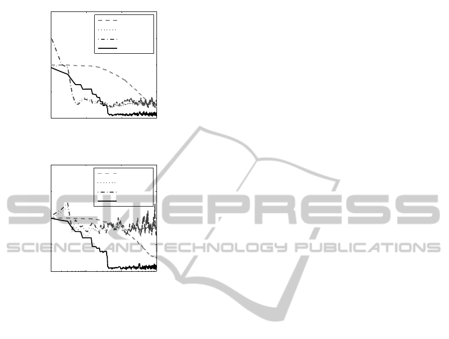
for the nonlinear case. In Figure 5 we can see the

learning curves of conventional linear TD(λ) (dashed

line), LSTD(λ) (dotted line), RLST(λ) (dotted dashed

line) and OSVR-TD (solid line). The RMS error

in these graphics are normalized with a RMS error

for initial VFA V = 0 for all states. In linear case,

Figure 5(a), although LSTD(λ) and RLST(λ) algo-

rithms convergeearlier than OSVR-TD algorithm, the

OSVR-TD algorithm had lower RMS error after con-

vergence. In nonlinear case, Figure 5(b), LSTD(λ)

and RLST(λ) algorithms could not have achieved sig-

niﬁcant results predicting the value function.

...

1112

rrrrr

Figure 4: A 13-state Markov chain (Boyan, 2002).

Table 1: Algorithms parameters.

Algorithm γ λ α

(0)

TD(λ) 1.0 0.4 0.01 1000

LSTD(λ) 0.9 0.9 - -

RLSTD(λ) 0.9 0.3 - -

OSVR-TD 1.0 - 0.8 -

Table 2: Performance comparison between TD(λ),

LSTD(λ), RLSTD(λ) and OSVR-TD.

(a) Linear Hop-World

Algorithm

Episodes

10 100 100

TD(λ) 13.89 10.69 3.10

LSTD(λ) 5.40 3.36 3.87

RLSTD(λ) 5.11 3.87 5.16

OSVR-TD 7.73 0.99 1.06

(b) Nonlinear Hop-World

Algorithm

Episodes

10 100 100

TD(λ) 67.45 53.77 17.21

LSTD(λ) 46.12 57.47 55.33

RLSTD(λ) 52.64 60.22 47.67

OSVR-TD 43.04 3.80 4.61

6 CONCLUSION

This paper proposes a new method of VFA for TD

learning based on OSVR models. Compared to tra-

ditional algorithms TD(λ), LSTD(λ) and RLSTD(λ),

it has signiﬁcant values for nonlinear approximation

abilities. The OSVR-TD has been applied success-

fully both to linear and nonlinear Hop-World prob-

lems. In addition to having achieved better results

than other algorithms, no featurization is necessary

in the state space, in spite of the necessary tuning of

the OSVR model parameters. More theoretical and

experimental analysis on the OSVR-TD algorithm as

well an extension to learning control problems is our

ongoing work.

ACKNOWLEDGEMENTS

The authors acknowledge CAPES for the support.

ICINCO2015-12thInternationalConferenceonInformaticsinControl,AutomationandRobotics

322

0.5

1.5

Episodes

RMS error

Linear HopWorld

TD(λ)

LSTD(λ)

RLSTD(λ)

OSVR−TD

(a) Linear Hop-World

0.5

1.5

Episodes

RMS error

Nonlinear HopWorld

TD(λ)

LSTD(λ)

RLSTD(λ)

OSVR−TD

(b) Nonlinear Hop-World

Figure 5: Performance comparison between TD(λ),

LSTD(λ), RLSTD(λ) and OSVR-TD.

REFERENCES

Bellman, R. E. (1957). Dynamic programing. Princeton

University Press, Princeton, NJ.

Bertsekas, D. P. and Tsitsiklis, J. N. (1996). Neuro-Dynamic

Programming. Athena Scientiﬁc, Nashua, NH, 1st

edition.

Boyan, J. A. (2002). Technical update: Least-squares tem-

poral difference learning. Machine Learning, 49:233–

246.

Bus¸oniu, L., Babuˇska, R., Schutter, B. D., and Ernst,

D. (2010). Reinforcement Learning and Dynamic

Programming Using Function Approximators. CRC

Press, Inc., Boca Raton, FL, USA.

Cortes, C. and Vapnik, V. (1995). Support vector networks.

Machine Learning, 20:273–297.

Cristianini, N. and Shawe-Taylor, J. (2000). An Introduction

to Support Vector Machines: And Other Kernel-based

Learning Methods. Cambridge University Press, New

York, NY, USA.

Drucker, H., Burges, C. J. C., Kaufman, L., Smola, A.,

and Vapnik, V. (1997). Support vector regression ma-

chines. Advances in neural information processing

systems, (9):155–161.

Lewis, F. L. and Vrabie, D. (2009). Reinforcement learn-

ing and approximate dynamic programming for feed-

back control. IEEE Circuits and Systems Magazine,

9(3):32–50.

Liu, D. and Zhang, H. (2005). A neural dynamic program-

ming approach for learning control of failure avoid-

ance problems. Intelligent Control and Systems, In-

ternational Journal of, 10(1):21–32.

Ma, J., Theiler, J., and Perkins, S. (2003). Accurate on-

line support vector regression. Neural Computation,

15(11):2683–2704.

Martin, M. (2002). On-line suport vector machines for func-

tion approximation. Software Department, Universi-

tat Polit`ecnica de Catalunya, Technical Report(LSI-

02-11-R):1–11.

Powell, W. B. (2011). Approximate Dynamic Program-

ming: Solving the Curses of Dimensionality. Wiley,

Hoboken, 2nd edition.

Sch¨olkopf, B. and Smola, A. J. (2001). Learning with Ker-

nels: Support Vector Machines, Regularization, Opti-

mization, and Beyond. MIT Press, Cambridge, MA,

USA.

Smola, A. J. and Sch¨olkopf, B. (2004). A tutorial on

support vector regression. Statistics and Computing,

14(3):199–222.

Sutton, R. S. (1988). Learning to predict by the method of

temporal differences. Machine Learning, 3:9–44.

Sutton, R. S. and Barto, A. G. (1998). Reinforcement Learn-

ing, An Introduction. MIT Press, Cambridge, MA,

USA, 1st edition.

Szepesv´ari, C. (2010). Algorithms for Reinforcement

Learning. Morgan & Claypool Publishers, Alberta,

Canada.

Tsitsiklis, J. N. and Roy, B. V. (1997). An analysis of

temporal-difference learning with function approxi-

mation. IEEE Transactions on Automatic Control,

42(5):674–690.

Vapnik, V. N. (1995). The nature of statistical learning the-

ory. Springer-Verlag, New York.

Wang, F. Y., Zhang, H., and Liu, D. (2009). Adaptive dy-

namic programming: An introduction. IEEE Compu-

tational Intelligence Magazine, 4(2):39–47.

Xu, X. (2006). A sparse kernel-based least-squares tem-

poral difference algorithm for reinforcement learning.

Proceedings of the Second International Conference

on Advances in Natural Computation, Part I:47–56.

Xu, X., gen He, H., and Hu, D. (2002). Efﬁcient reinforce-

ment learning using recursive least-squares methods.

Artiﬁcial Intelligence Research, Journal of, 16:259–

292.

Xu, X., Zuo, L., and Huang, Z. (2014). Reinforcement

learning algorithms with function approximation: Re-

cent advances and applications. Information Sciences,

261:1–31.

Temporal-DifferenceLearning-AnOnlineSupportVectorRegressionApproach

323