Multi-objective Optimization for Control and Process Operation

Helem Sabina S

anchez and Ramon Vilanova

Departament de Telecomunicaci

o i Enginyeria de Sistemes, Universitat Aut

onoma de Barcelona,

08193 Bellaterra, Barcelona, Spain

1 STAGE OF THE RESEARCH

It is well known, that satisfying the requirements

and constraints required by a control engineering sys-

tem in many cases is a difﬁcult task to fulﬁlling for

each of the objectives. Owing to this, this research

aims to apply the Multi-objective Optimization De-

sign (MOOD) procedure to PID controller tunning by

means Multi-Objective Optimization based on deter-

ministic algorithm. This procedure is focus on pro-

vide reasonable trade-off solution among the objec-

tives in conﬂictive. Currently, we are working on con-

tribution based on: an approach on the MOO pro-

cess for PI controller, applying the methodolgy to

Fractional-order PID controllers and doing a research

stay at the University of Brescia (UNIBS), Italy.

2 OUTLINE OF OBJECTIVES

The following aims are deﬁned for the development

of this research:

• First Year:

– Review of the state of art. Existing methods

and approaches for the planning and the deﬁni-

tion of a Multi-Objective Optimization (MOO)

process and MOOD procedure. To have an idea

of the work done and the work to be done.

– Identifying methodologies and tools needed to

solve optimization problems. Test differents al-

gorithms according to the preferences.

– Limitations on the search domain and func-

tional constraints linked to the operation of the

system.

– Select the methodology (algorithm and the de-

cision making technique).

• Second Year:

– Applications on controller tunning: PI, PID

controlllers (set-point step response).

– Consider both operation modes (set-point and

load disturbance).

– Collaborative work with others research group

dedicate to Optimization.

• Currently:

– Contribution on MOO process (new methodol-

ogy).

– Validation of the new methodology (bench-

mark, FOPID and others).

3 RESEARCH PROBLEM

This proposal seeks to develop a methodology to ad-

dress issues of control and operation of processes by

implementing a MOOD procedure. In a control sys-

tem there are different measures and indexes that are

made in order to measure their performance. Satisfy-

ing the speciﬁcations and constraints required is of-

ten a challenge. Sometimes, the improvement in per-

formance of one of them is at the expense of wors-

ening another. This kind of problems where the de-

signer have to deal with the fulﬁllment of multiple

objectives are known as Multi-Objective Problems

(MOPs). Such problems can be addressed using a si-

multaneous optimization of all targets. This implies

to seek for a Pareto optimal solution which the objec-

tives have been improved as possible without giving

anything in exchange. To guarantee the overall per-

formance of a MOOD procedure the following steps

are necessary: 1) deﬁnition of the MOP, 2) the MOO

process to approximate the so-called Pareto set and 3)

a Multi-criteria Decision Making (MCDM) is carried

out in order to implement the most preferable solu-

tion from the set. The MOOD procedure brings to the

designer the possibility to appreciate the trade-off of

the objectives (conﬂictive) this characteristic can be

useful for controller tunning.

4 STATE OF THE ART

The design of a PI-PID control system starts from a

model of the process to be controlled and a set of re-

Sabina Sánchez H. and Vilanova R..

Multi-objective Optimization for Control and Process Operation.

 2015 SCITEPRESS (Science and Technology Publications, Lda.)

quirements to be satisﬁed. These requirements often

enter into conﬂict making the task of ﬁnding the ap-

propriate controller parameters not an easy task. It is

on that basis that constrained optimization can enter

into play by helping to delimit the tradeoff between

possible conﬂicting requirements. Such requirements

use to be the conﬂicting performance and robustness

speciﬁcations (in the different forms that they can be

established). Typical control system requirements in-

clude performance speciﬁcations on load disturbance

attenuation, robustness, control input usage, set-point

response and measurement noise. It is a fact that dis-

turbance rejection is of primary interest in process

control, where what really matters is steady-state reg-

ulate. On the other hand set-point changes are likely

to occur. In such cases it is possible to tackle them by

using an appropriate two-degree-of-freedom (2-DoF)

architecture. Therefore, when introducing time re-

sponse performance requirements we can conﬁne our-

selves to disturbance attenuation. In fact, as a feed-

back property, disturbance attenuation will enter into

conﬂict with robustness as both are determined by

the controller parameters that appear in the feedback

loop. From a purely optimization problem point of

view, all such requirements could be used to establish

the set up of a Multiobjective Optimization Problem

(MOP). In some cases, the high performance is not

compatible with a robust controller for process vari-

ations. The controller design can be viewed as the

search for the best compromise between all the spec-

iﬁcations and thereby the idea of multiobjective opti-

mization (MOO) can be an alternative to resolve this

problem (Mart

ınez et al., 2006). MOO provides the

possibility of a better selection of the ﬁnal solution as

there is no part ignored in the search space. The ﬁnal

solutions (Pareto set), represents the whole space of

the design variables and their projection in the space

of objectives as the Pareto front.

4.1 Multi-objective Optimization -MOO

A multi-objective optimization problem (MOP) can

be handled by performing a simultaneous optimiza-

tion of all objectives. This implies the existence of a

set of solutions, where no one is better than the oth-

ers, but differ in the degree of performance between

the objectives (Miettinen, 1998). This set of solutions

will offer a higher degree of ﬂexibility at the decision

making stage. The role of the designer is to select the

most preferable solution according to his (her) needs

and preferences for a particular situation. A MOP,

without loss of generality (since a maximization prob-

lem can be converted to a minimization problem), can

be stated as follows:

min

θ∈ℜ

J (θ) = [J

(θ), . . . , J

(θ)] ∈ ℜ

(1)

Therefore a set of Pareto-optimal solutions is de-

ﬁned as the Pareto set Θ

and its projection into

the objective space is known as the Pareto front J

Where each solution in the Pareto front is said to be a

non-dominated and Pareto-optimal solution. In gen-

eral, it does not exist a unique solution because there

is not a solution better than other in all the objectives.

MOO techniques search for a discrete approxima-

tion Θ

∗

of the Pareto set Θ

capable of generate a

good quality description of the Pareto front J

∗

. In

this way, the decision maker (or simply the designer)

can analyze the set and select the most preferable so-

lution.

A general framework is required to successfully

incorporate the MOO approach into any engineering

process. A multiobjective optimization engineering

design (MOOD) methodology consists (at least) of

three main steps (Reynoso-Meza et al., 2014b): the

MOOP deﬁnition (objectives, decision variables and

constraints), the MOO process (optimizer selection)

and the decision-making (DM) stage (analysis and se-

lection of the calculated solutions).

4.2 Multiobjective Problem Deﬁnition

Requirements often include speciﬁcation on load dis-

turbance compensation, set-point following and ro-

bustness to process uncertainty.

Reasonably the most basic MOP statement for

PID controller tuning goals could be represented as:

= [K

, T

] (2)

Where θ

are the parameters of the optimal PID con-

troller.

minJ (θ

) = [J

(θ

), J

(θ

)] (3)

(θ

) = Per f ormance(θ

)

(θ

) = Robustness(θ

)

Control performance J

(θ

) can be characterized by

the integrated absolute error

IAE =

∞

e(t)

dt, (4)

where e is the control error due to a unit step load dis-

turbance. It is a good performance measure for con-

trol system with integral action.

In order to measure the smoothness of the control ac-

tion we have the control signal total variation J

(θ

)

is deﬁned as

∞

∑

k=1

u(k + 1) − u(k) (5)

ICINCO2015-DoctoralConsortium

The maximum sensitivity is an indication of the sys-

tem robustness (relative stability):

= max



1 +C

( jw)P( jw)



(6)

where C

is the feedback controller transfer function,

P is the controlled process.

In some experiments we propose to use the inte-

grated square error (ISE) as a measure of performance

for the set-point and load disturbance step responses

(as in (Arrieta et al., 2010)) and the maximum sensi-

tivity (6) as a constraint of MOOP.

ISE

∞

(t)dt, d = 0 (7)

is the integrated square error when a set-point step

response is considered,

ISE

∞

(t)dt, r = 0 (8)

5 METHODOLOGY

In this section a brief description about the algorithms

used to calculated the Pareto front approximation and

the MCDM technique implemented to select a trade-

off point from the Pareto front as the ﬁnal solution

to the MOP. Both of them have shown to be useful

for PI and PID controllers in (S

anchez and Vilanova,

2013a; S

anchez and Vilanova, 2013b; S

anchez and

Vilanova, 2014; S

anchez et al., 2014; Reynoso-Meza

et al., 2014a; S

anchez et al., 2013).

5.1 Normal Normalized Constraint for

Multi-objective Optimization

This algorithm is used to determine the Pareto front

and the set of optimal solutions. Using this algo-

rithm, the optimization problem is separated into sev-

eral constrained single optimization problems. After

series optimizations, a set of evenly distributed Pareto

solutions results. The NNC method incorporates a

critical linear mapping of the design objectives. This

mapping has the desirable property that the resulting

performance of the method is entirely independent

of the design objectives scales and in the ability to

generate a well distributed set of Pareto points even

in numerically demanding situations (Messac et al.,

2003b). The NNC method is presented here to solve

a bi-objectives problem, but it can be generalized to

n-objectives. An extract of the algorithm is presented,

for more details about the method see (Messac et al.,

2003a). The algorithm is available in Matlab Central.

1 Generate the anchor points J|

(x) for each

objective;

2 Calculate the Utopian Point and NADIR;

3 Normalized the objective space;

4 Generate the utopian hyperplane;

5 Deﬁnition of the normalized increments;

6 Generate the utopian lines;

7 while normalized increments do

8 Optimize;

9 end

10 Algorithm concludes. J

is approximated by

∗

= A|

;

Algorithm 1: NNC Algorithm outline.

5.2 Nash Solution-NS

All the points of the Pareto front are equally accept-

able solutions. Thus, there is the need to choose one

of such point as the ﬁnal solution to the MOOP. This

is the last part of the MOOD procedure, the decision-

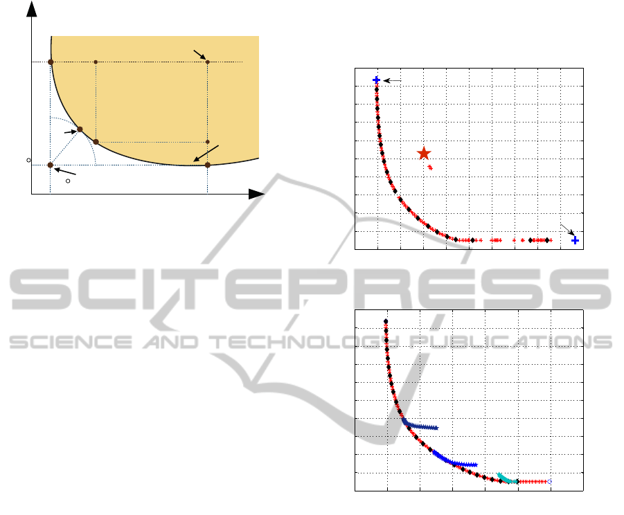
making stage. For this purpose we propose the Nash

(NS) criteria, for which a graphical explanation can

be seen in Figure 1. In order to understand this op-

tion, we introduce what can be called the disagree-

ment point. If we think on both objectives indepen-

dently, none of them would agree on this point as a

common solution because it represents the worst sit-

uation. In addition, this selection can be improved

with respect of both objectives. On that basis, the

area of the rectangle deﬁned by the points (NS, A,

B) and the disagreement point provides a measure of

the amount of solutions the NS point improves with

respect to both objectives simultaneously. The NS is

the solution that maximizes such area, this denomi-

nation comes from identifying this point as the Nash

Solution on a bargaining game among both objectives

(Aumann and Hart, 1994).

6 EXPECTED OUTCOME

This thesis contains a research line in MOO process,

focuses on controller tunning applications. For this

reason it is expecting the following contributions:

• Cover the theorical background required for this

thesis.

• Develop a methodology to apply for the controller

tunning (algorithm and MCDM technique).

Multi-objectiveOptimizationforControlandProcessOperation

J J

1 1

ANS

Disagreement Point

Utopia point

Pareto

front

Figure 1: The Nash solution for a bi-objective case.

• Identify gaps that exist on the methodologies of

the MOOD procedure.

• Applying the selected tools for the controller

tunning: 1) Proportional-Integral (PI) con-

trollers, 2) Proportional-Integral-Derivative (PID)

controllers, 3) Fractional-Order Proportional-

Integral-Derivative (FOPID) controllers.

• Implement the MOOD procedure in case of stud-

ies (benchmark).

• Develop proposals on tools to improve the usua-

bility and performance of the MOOD procedure.

• Nevertheless, during the develop of this thesis:

collaborations with other research groups it will

be carried out.

• Publishing the results.

This thesis is dedicated to ﬁnd the methodology

and techniques to address problems of control and op-

eration of processes through the application of multi-

objective optimization strategies. Some of the contri-

butions are listed bellow.

6.1 Correlation Between TV and M

anchez and Vilanova, 2013a)

Figure (2) shows the pareto front that results for a pro-

cess model with K = 1 and τ

= 0.5. Anchor points

and the location of a Ziegler-Nichols tuning are also

shown. In this case, we do not have any constraint on

the robustness. Just performance is considered.

Instead, if we add as a robustness constraint, three

usual values for M

, for example M

= {1.4, 1.6, 1.8};

what we are doing is constraining the achievable sys-

tem performance. This is shown in ﬁgure (3), where

the new Pareto sets corresponding to each one of the

robustness levels are jointly shown with the uncon-

strained one. As it is seen, we get a new pareto front,

considerably smaller than the previous one, constrain-

ing ourselves to a really small set of possible solu-

tions.

0.4 0.5 0.6 0.7 0.8 0.9 1 1.1 1.2 1.3

0.06

0.07

0.08

0.09

0.1

0.11

0.12

0.13

0.14

0.15

0.16

IAE

Pareto front

Anchor

Point

Anchor

Point

Figure 2: Pareto front for K = 1 and τ

= 0.5.

0.4 0.5 0.6 0.7 0.8 0.9 1

0.06

0.07

0.08

0.09

0.1

0.11

0.12

0.13

0.14

0.15

0.16

IAE

Ms=1.8

Ms=1.6

Ms=1.4

Figure 3: Comparison of Pareto fronts.

Therefore, there is a correlation between the value

of M

and the control input usage in terms of TV . Ef-

fectively, as pointed out in (Foley et al., 2005) there

do exists a correlation. This is clearly shown in ﬁg-

ure (4) for the example at hand. We can therefore di-

rectly associate the robustness to the TV performance

index and think on that index not just as the input us-

age but also as a measure of the closed system ro-

bustness. From ﬁgure (4) the approximate relation is

established M

≈ 10.5TV + 0.77. This allows to think

on the multi objective optimization problem simply as

a tradeoff between TV and J

IAE

, having in mind that

the selection of the appropriate point form the pareto

front will need to take into account the level of robust-

ness we need (lower values for TV ). Effectively this

simpliﬁes the setup for the optimization problem and

subsequent generation of the pareto front.

ICINCO2015-DoctoralConsortium

0.06 0.07 0.08 0.09 0.1 0.11 0.12 0.13 0.14 0.15 0.16

1.4

1.5

1.6

1.7

1.8

1.9

2.1

2.2

2.3

2.4

Figure 4: TV and M

correlation, M

≈ 10.5TV + 0.77.

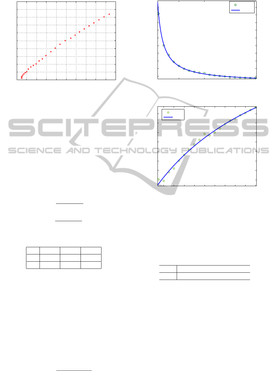
6.2 Nash-based PI Tuning (S

anchez and

Vilanova, 2013b)

The values of τ

are selected to take the FOPDT pro-

cesses with small, medium and fairly long dead time

into account, the values of the normalized dead-time

(τ

) are considered from 0.1 to 2. To obtain appropri-

ate values of κ

and τ

for a speciﬁed value of τ

, non-

dominated solutions are determined using the NNC

method. Finally, when we obtain the Pareto front one

optimal solution is choosen known as Nash solution.

The tuning formulae is as follows:

∗ τ

+ a

+ b

, (9)

∗ τ

+ a

+ b

, (10)

Table 1: Controller constants for κ

and τ

0.098 0.565 0.026

2.624 1.548 2.649

The constants in equations (9-10) are shown in Ta-

ble 1. The ﬁtting obtained using this formulae are also

shown in ﬁgures (5-6).

6.3 Comparison Between

Multi-objective Optimization

Techniques (S

anchez and Vilanova,

2014)

Consider the four-order controlled benchmark pro-

cess proposed in (

Astr

om and H

agglund, 2000) and

given by the transfer function

(s) =

∏

n=0

(α

s + 1)

(11)

0.5 1 1.5 2

0.5

1.5

2.5

3.5

4.5

vs. τ

fit

Figure 5: Normalized controller gain.

0.2 0.4 0.6 0.8 1 1.2 1.4 1.6 1.8 2

0.7

0.8

0.9

1.1

1.2

1.3

1.4

vs. τ

fit

Figure 6: Normalized controller integral time.

with α ∈

{

0.1, 0.5, 1.0

}

. Using the three-point identi-

ﬁcation procedure 123c (Alfaro, 2006) FOPDT mod-

els have been obtained whose parameters are shown

in Table 2. These models will be used for PI con-

troller design.

Table 2: Example - FOPDT Models.

α K T L τ

0.50 1 1.247 0.691 0.554

• Case 1: The pareto front was obtained using the

NNC and a reference point (Ziegler-Nichols as a

initial point), using the ZN tunning rule (K

1.62T

= 2.30), this solution is dominated by other

solutions as we can see in ﬁgure (7)

• Case 2: The pareto front was calculated with the

Multiobjective Differential Evolution Algorithm

with Spherical Pruning (sp-MODE) using perti-

nence criteria. This concept refers to the abil-

ity to give a practical solution from the point of

view of the designer. In this case, the Pareto front

is bounded, if it is known a priori which solu-

tions are looking for and are interesting for the

Multi-objectiveOptimizationforControlandProcessOperation

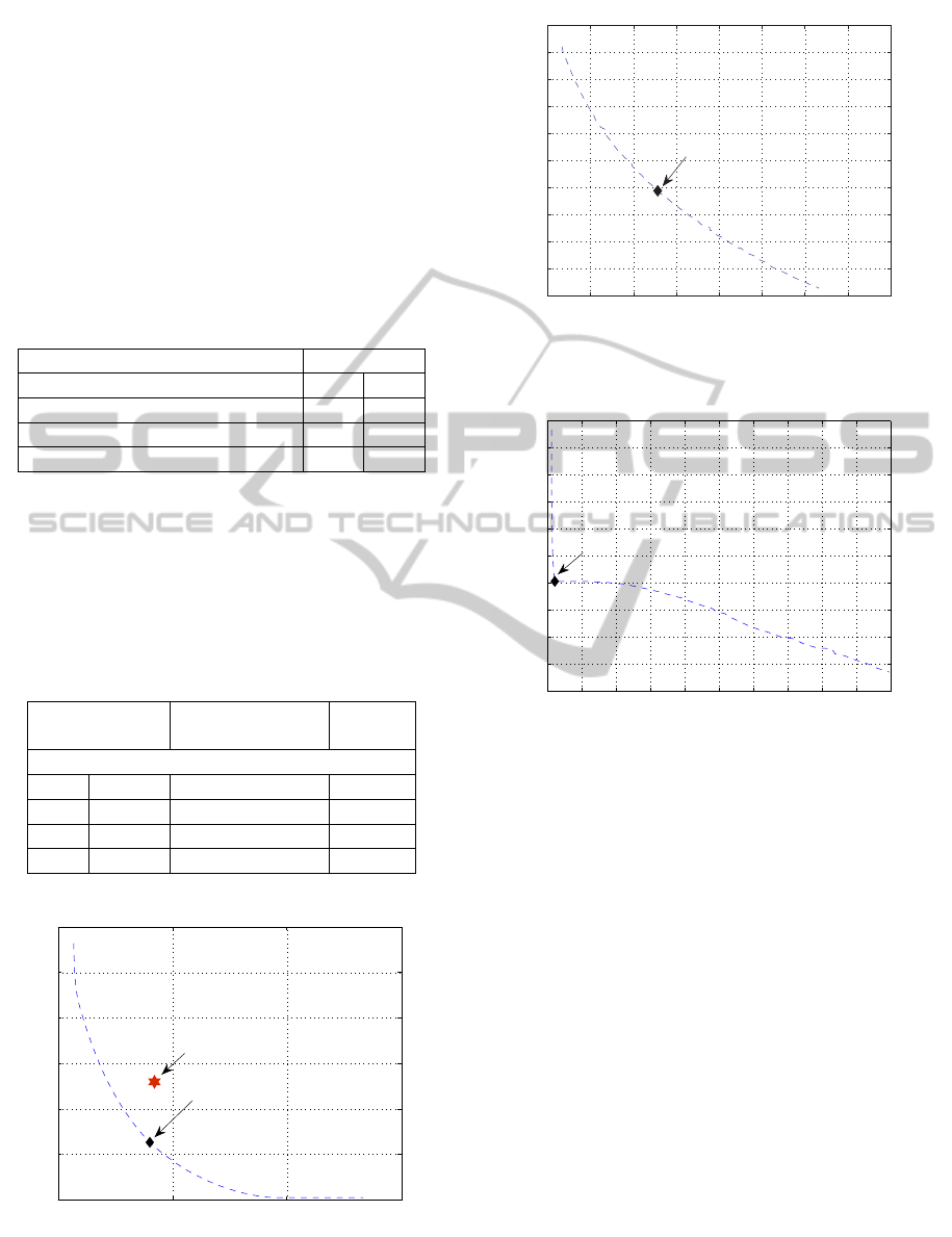
designer. It is a useful option when you know that

in some cases, improving one objective does not

justify the severe degradation in the other. The

values (IAE = 0.9217 TV = 0.1319) were used as

the pertinence criteria. They were calculated with

the parameters mentioned before. In ﬁgure (8) it

is possible to see how the algorithm focuse the

search only in the range that contains the values

of pertinence.

• Case 3: We use the sp-MODE but this time with-

out of pertinence, see ﬁgure (9).

Table 3: Example - Controller Parameters.

α = 0.5

Methods Kp Ti

Case 1: NNC 1.34 1.86

Case 2: sp-MODE (pertinence) 1.05 1.18

Case 3: sp-MODE 0.84 1.37

For each one of these cases the Nash solution was

calculated, therefore in Table 3 the parameters of the

controller (PI) are shown and in Table 4 the values

of performance and robustness of the system are dis-

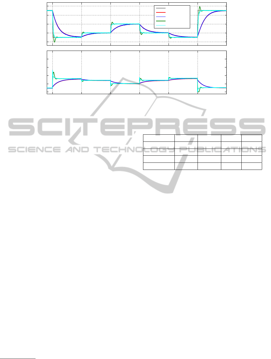
played. Furthermore, ﬁgure (10) shows the achieved

time response when facing a step load-disturbance.

Table 4: Example - Performance and Robustness.

Case 1 Case 2 Case 3:

NNC sp-MODE (pertinence) sp-MODE

0=0.5

IAE 0.9022 0.7662 1.0601

TV 0.1023 0.1118 0.0856

1.64 1.67 1.44

max

0.3016 0.3167 0.3446

0.5 1 1.5 2

0.08

0.1

0.12

0.14

0.16

0.18

0.2

NASH

IAE

Pareto Front (model corresponding to α=0.5)

Figure 7: Pareto front for the process model corresponding

to α = 0.5 (Case 1).

0.65 0.7 0.75 0.8 0.85 0.9 0.95 1

0.085

0.09

0.095

0.1

0.105

0.11

0.115

0.12

0.125

0.13

0.135

IAE

Frente de Pareto (modelo correspondiente a =0.5)

NASH

Figure 8: Pareto front for the process model corresponding

to α = 0.5 (Case 2).

0 5 10 15 20 25 30 35 40 45 50

0.02

0.04

0.06

0.08

0.1

0.12

0.14

0.16

0.18

0.2

IAE

Pareto Front (model corresponding to α=0.5)

NASH

Figure 9: Pareto front for the process model corresponding

to α = 0.5 (Case 3).

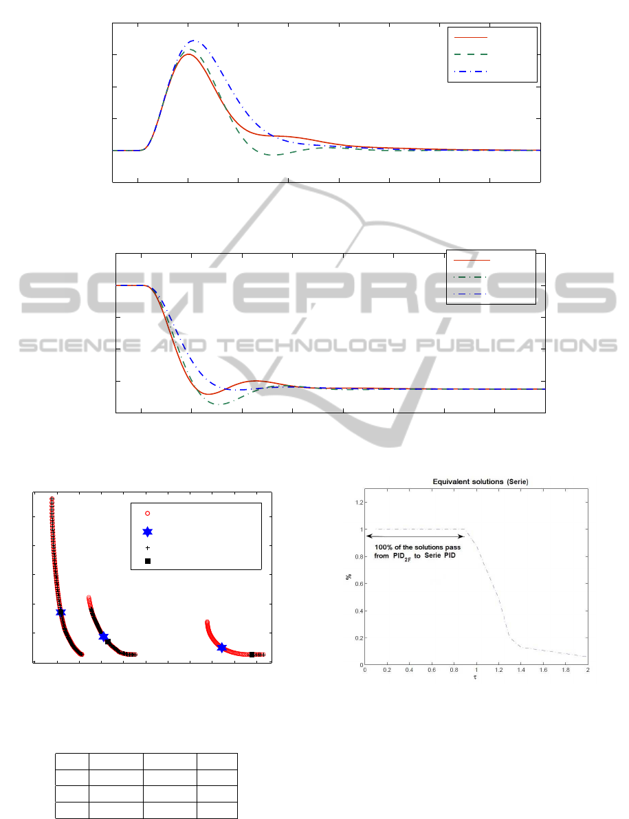
6.4 Equivalence and Optimality for PID

Controllers (S

anchez et al., 2014)

Based on the initial work of ((Alfaro and Vilanova,

2012)) where the differet formulations for PID con-

trollers are listed and conversion formulae is pro-

vided, the equivalence between them, is analyzed

here.

The optimization was applied to the most gen-

eral conﬁguration PID

from τ = [0.1 − 2.0]. Here

we only present 3 representative cases of τ =

[0.6, 1.0, 2.0], the Pareto front is shown in Figure 11.

It can be seen that when the normalized dead time in-

creases the IAE index as well.

Furthermore, the total variation (TV) is decreasing

while also the robustness of the system is higher. In

((S

anchez and Vilanova, 2013a)) some experiments

shows that there is correlations between both of them.

This can be see in Table (5-6), where the values of

performance and robustness are shown for each con-

ﬁguration and its respective τ. In Figure (11) is also

ICINCO2015-DoctoralConsortium

10 12 14 16 18 20 22 24 26

−0.1

0.1

0.2

0.3

0.4

y(t)

Output to a unit load−disturbance

t(s)

Case 1

Case 2

Case 3

10 12 14 16 18 20 22 24 26

−0.8

−0.6

−0.4

−0.2

0.2

t(s)

Control Signal

u(t)

Case 1

Case 2

Case 3

Figure 10: Time output and control responses for α = 0.5.

0.2 0.4 0.6 0.8 1 1.2 1.4 1.6 1.8 2 2.2

0.06

0.08

0.1

0.12

0.14

0.16

IAE

Pareto Fronts and Nash Solutions

Ideal with Filter (PID

Nash Solution (PID

Equivalent Serie

Nash Solution (Serie)

Figure 11: Pareto Front and Nash Solution.

Table 5: Performance and Robustness (PID

y PID

IAE TV M

0.6 0.4348 0.0940 1.69

1.0 0.8571 0.0740 1.51

2.0 2.1583 0.0650 1.42

shown the Series equivalent for PID

y PID

It is worth mentioning, that when it passed from

Figure 12: Equivalent solutions from a PID

to Serie PID.

PID

conﬁguration to the PID

, all the solutions had

the equivalent; owing to this both conﬁgurations have

the same Nash solution. In Figure (12) we see that

the equivalent solutions for the series conﬁguration

are less as τ increases, in this cases the Nash solutions

will not be the same for the Series PID see Table (6).

Multi-objectiveOptimizationforControlandProcessOperation

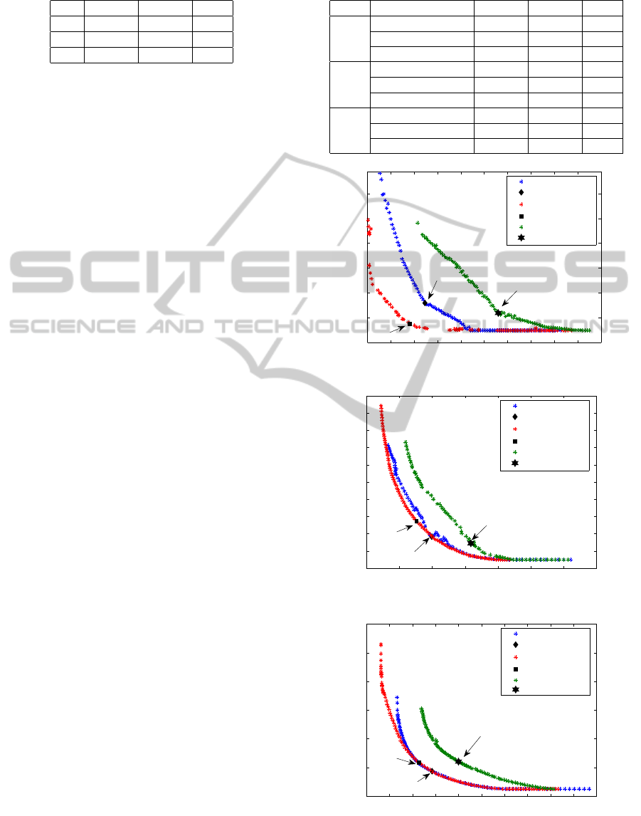
Table 6: Performance and Robustness (Serie).

IAE TV M

0.6 0.4348 0.0940 1.69

1.0 0.8206 0.0773 1.53

2.0 1.8869 0.0697 1.48

6.5 Optimality Comparison of PID

Implementations (S

anchez and

Vilanova, 2014)

The Pareto front for each conﬁguration was calculated

with normalized dead times from 0.1 to 2.0. But in

this paper only three representative cases (0.1, 0.75

and 1.75) are presented. The Pareto fronts are shown

in ﬁgure 13.

The displacement of the Pareto fronts of each con-

ﬁguration shows the behavior of the PID algorithm

from a general to a more constrained PID conﬁgura-

tion. As it can be seen as the τ

increases, the Pareto

fronts; Figure (13); are getting closer between each

other but always dominated by the PID

conﬁgura-

tion. The superiority of this conﬁguration regarding

the Standard one increases as τ

decreases. However

both conﬁgurations show a clear superiority with re-

spect to the series one. As shown in Table (7) the

values of performance and robustness for each case

are different, sometimes the 2DoF PID Standard and

Ideal with ﬁlter have similar values compared to the

Series conﬁguration.

With the experiments performed in this work we

realized that if we want a better functionality, it is

not necessary to use the conversion formulae. For ex-

ample see in Figure (13a), if we apply the equations

to the 2DoF Series conﬁguration in order to obtain

a PID

, the results of the performance and robust-

ness will be the same as the 2DoF Series (the new

Pareto front calculated would be at the same position

as the Series conﬁguration). This means that instead

of applying the conversion formulae we could tune

the controller again in order to obtain a better perfor-

mance, robustness and also less overshoot. Overall,

this representation by the Pareto front allows us to see

how important is to see the behavior of this indexes

(IAE, TV, M

6.6 Reliability based Multiobjective

Optimization Design Procedure for

PI Controller Tunning

(Reynoso-Meza et al., 2014a)

This was a collaborative work, we presented a MOOD

procedure involving a reliability based MOOP state-

Table 7: Controller performance.

Controller IAE TV M

0.1

Standard 1.3534 0.1725 1.51

Series 1.4007 0.1679 1.46

Ideal with Filter 1.3365 0.1713 1.44

0.75

Standard 2.7298 0.1994 1.53

Series 3.2146 0.1774 1.52

Ideal with Filter 2.5964 0.2197 1.62

1.75

Standard 5.3946 0.1876 1.57

Series 5.9093 0.1913 1.58

Ideal with Filter 5.2701 0.1986 1.67

0.095 0.1 0.105 0.11 0.115 0.12 0.125 0.13 0.135 0.14 0.145

0.064

0.066

0.068

0.07

0.072

0.074

0.076

IAE

Standard

=1.51

Ideal with Filter (ID

)

=1.44

Series

=1.46

Standard

Series

(a) Pareto Front τ

= 0.1

0.4 0.5 0.6 0.7 0.8 0.9 1 1.1

0.06

0.07

0.08

0.09

0.1

0.11

0.12

0.13

0.14

0.15

0.16

IAE

Standard

=1.53

Ideal with filter (ID

)

=1.62

Series

=1.52

Series

Standard

(b) Pareto Front τ

= 0.75

1.3 1.4 1.5 1.6 1.7 1.8 1.9 2 2.1 2.2

0.06

0.08

0.1

0.12

0.14

0.16

0.18

IAE

Standard

=1.57

Ideal with filter (ID

)

=1.67

Series

Ms=1.58

Standard

Series

= 1.75

Figure 13: Pareto Front for differents τ

ICINCO2015-DoctoralConsortium

100 200 300 400 500 600 700

−10

−5

Temperature [ºC]

100 200 300 400 500 600 700

100

Time [sec]

U [%]

Reference

Controller IS

Controller NS−2D

Controller NS−3D

Controller LD−3D

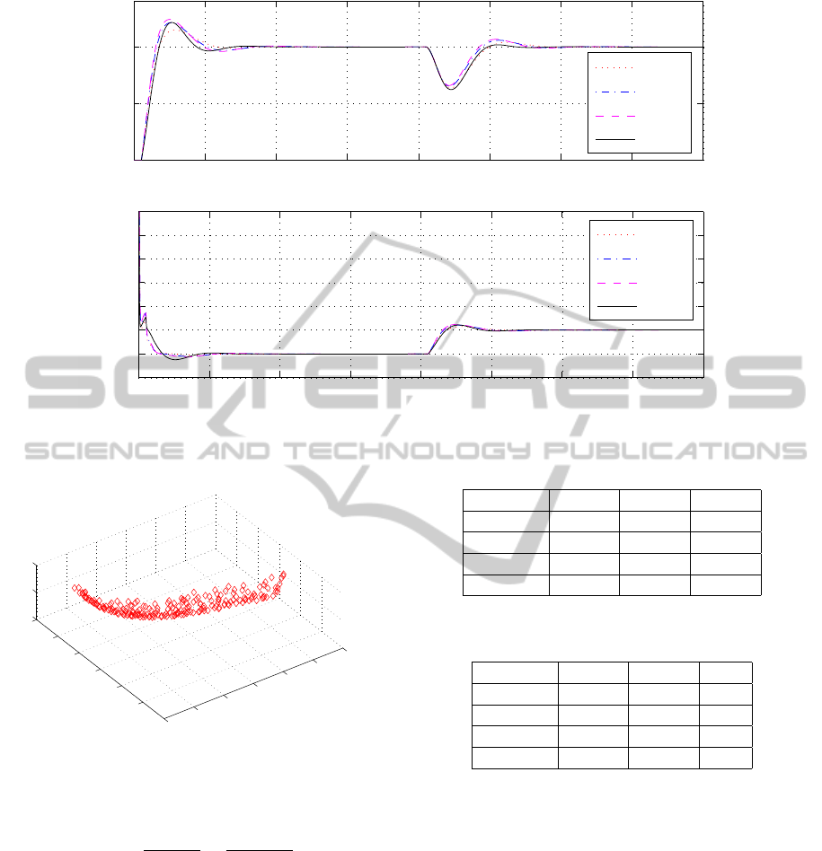
Figure 14: Performance comparison on the Peltier Cell.

ment for controller tuning. To improve the results

in the MOO process an hybrid approach has been

proposed to calculate the Pareto front approximation.

Merging deterministic and evolutionary algorithms,

the Normalized Normal Constraint (NNC) and the

Multiobjective Differential Algorithm with Spherical

Pruning (sp-MODE), respectively. A Peltier cell was

chosen to evaluate the above, mentioned MOOD pro-

cedure. First we generate the preliminary bi-objective

Pareto front J

0∗

with the NNC algorithm. With such

Pareto front, two solutions are selected for further

evaluation: the initial solution employed in the op-

timization process and the Nash-based (IS

and NS-

respectively). In the execution using the sp-

MODE and the Pareto front approximation from NNC

algorithm, pertinency is included in the algorithm to

bound the new objective using the starting solution

of the NNC algorithm. Two solutions were selected:

Nash-based and a solution selected by analyzing the

Pareto front using Level diagrams (NS-3D and LD-

3D respectively).

The performance of the selected controllers is

shown in Figure (14) and in Table (8). Whilst per-

formance of controllers IS and NS-2D are similar it is

interesting to notice differences between controllers

NS-2D and NS-3D. Both of them have been selected

using the same Decision Making (DM) rule (Nash so-

lution). Differences on the performance are due to

the additional information used in the MOP statement

minding degradation on IAE performance. Controller

LD-3D selected from the LD visualization is consis-

tent with the fact of improving IAE at expense of

more control effort (TV). The results presented val-

idate the procedure as useful for PI tuning of non-

linear systems.

Initial Solution

Nash Solution in 2D

Table 8: Controller performance on the Peltier cell case

study.

Controller K

IAE TV

IS 0.19 2.74 992.4 86.0

NS-2D 0.1898 2.6613 967.6 86.8

NS-3D 0.5091 0.4057 154.6 263.9

LD-3D 2.3735 3.2623 120.7 657.4

6.7 Nash Solution for Optimal Balance

of Servo/Regulation Operation in

PID Control (S

anchez et al., 2015)

A multi-objective optimization approach is proposed

for the tuning of one degree-of-freedom proportional-

integral-derivative controllers where both the trade-

off between the servo and regulation operation modes

and the trade-off between performance and robustness

are considered. After having quantiﬁed the loss of

performance that occurs if robustness is taken into ac-

count in the optimal design of the controller, a tuning

rule is proposed based on the Nash solution, so that

a balanced robust tuning is obtained simply starting

from a ﬁrst-order-plus-dead-time model of the (self-

regulating) process.

It has been shown that, in this context, the robust-

ness of the system can be a critical issue and there-

fore it has to be included explicitly in the optimization

procedure. Tuning rules based on the Nash solutions

have also been devised so that the methodology can be

easily implemented in standard industrial controllers.

In this example we will illustrate how the imple-

mentation of the Nash tuning rules improves the ro-

bustness of the system and also maintains acceptable

values of the performance with respect to both the op-

eration modes. Consider the following process and

the corresponding FOPDT approximation ((Zhuang

Multi-objectiveOptimizationforControlandProcessOperation

0 5 10 15 20 25 30 35 40

0.5

Time

Process Variable

0 5 10 15 20 25 30 35 40

Time

Control Variable

α=0.25

α=0.50

α=0.75

Nash

α=0.25

α=0.50

α=0.75

Nash

Figure 15: Step responses for the illustrative example.

0.09

0.1

0.11

0.12

0.13

0.14

0.15

0.35

0.4

0.45

0.5

0.55

0.6

1.5

IAE

Pareto Front (τ

=0.1)

IAE

Figure 16: Pareto front for τ = 0.1.

and Atherton, 1993)):

P(s) =

−0.5s

(s + 1)

≈

−0.99s

1 + 1.65s

(12)

The PID controller parameters determined by us-

ing the Nash tuning rules and the intermediate tun-

ing rules ((Arrieta et al., 2010)) are shown in Table

(9) while the corresponding performance indices and

maximum sensitivity values are shown in Table 10.

The set-point and load disturbance step responses are

plotted in Figure (15).

From the results it can be seen that the perfor-

mance obtained with the Nash tuning is similar to

that obtained with the intermediate tuning despite the

maximum sensitivity is M

= 1.73 for the Nash tuning

while in the other cases it ranges from 2.26 to 2.77.

Table 9: PID controller parameters.

Tuning K

NS 1.9652 1.6477 0.3464

α = 0.25 1.791 1.378 0.520

α = 0.5 1.949 1.234 0.527

α = 0.75 2.016 1.177 0.531

Table 10: Performance and robustness value for the system

(12).

Tuning ISE

ISE

NS 0.2674 1.1511 1.73

α = 0.25 0.2562 1.1133 2.26

α = 0.5 0.2265 1.1793 2.59

α = 0.75 0.2172 1.2224 2.77

6.8 Future Work

The future research efforts will be conducted:

1. FOPID Controllers: to apply the same ap-

proach we use in (S

anchez et al., 2015) to

Fractional-order proportional-integral-derivative

(FOPID) controllers. A MOOD procedures will

be implemented to obtain a set of tuning rules for

FOPID controllers. Using the Nash solutions as

the MCDM technique. The tuning rules will be

devised in order to minimise the integrated abso-

lute error with a constraint on the maximum sen-

sitivity. The trade-off between the perfomance in

the set-point following and in the load disturbance

rejection task it will be taking into account, a pre-

liminary result is shown in Figure (16).

ICINCO2015-DoctoralConsortium

2. Multistage Procedure for PI Controller Tun-

ning: a multistage approach is proposed merg-

ing a deterministic and evolutionary algorithm,

the Normalized Normal Constraint (NNC) and

Multiobjective Differential Evolution Algorithm

with Spherical Pruning (sp-MODE), respectively.

This technique is formulated through design of a

multi-objective optimization procedure, to ensure

the construction of Pareto frontier that guarantee

well distribution and exclude the non-Pareto and

local Pareto points. This procedure focuses on

reliability-based optimization instances. To val-

idate the approach, we will consider the Boiler

Control Benchmark and the Peltier cell; the re-

sults of the improvement of the performance is

demonstrated and its usefulness for controller tun-

ing.

REFERENCES

Alfaro, V. M. (2006). Low-Order Models Identiﬁcation

from the Process Reaction Curve. Ciencia y Tec-

nolog

ıa (Costa Rica), 24(2):197–216. (in Spanish).

Alfaro, V. M. and Vilanova, R. (2012). Conversion for-

mulae and performance capabilities of two-degree-of-

freedom pid control algorithms. In Proceedings of the

17th. IEEE Conference on emerging technologies &

factory automation (ETFA).

Arrieta, O., Visioli, A., and Vilanova, R. (2010). Pid au-

totuning for weighted servo/regulation control opera-

tion. Journal of Process Control, 20(4):472–480.

Astr

om, K. J. and H

agglund, T. (5-7 April, Terrasa, Spain,

2000). Benchmark Systems for PID Control. In IFAC

Digital Control: Past,, Present and Future of PID

Control (PID’00).

Aumann, R. and Hart, S. (1994). Handbook of Game The-

ory with Economic Applications. Elsevier.

Foley, M., Ramharack, N., and Copeland, B. (2005). Com-

parison of PI controller tuning methods. Ind. Eng.

Chem. Res., 44(17):6741–6750.

Mart

ınez, M. A., Sanchis, J., and Blasco, X. (2006). Mul-

tiobjective controller design handling human prefer-

ences. Engineering applications of artiﬁcial intelli-

gence, 19(8):927–938.

Messac, A., Ismail-Yahaya, A., and Mattson, C. (2003a).

The normalized normal constraint method for gener-

ating the Pareto frontier. Structural and Multidisci-

plinary Optimization, (25):86 – 98.

Messac, A., Ismail-Yahaya, A., and Mattson, C. A. (2003b).

The normalized normal constraint method for gener-

ating the pareto frontier. Structural and multidisci-

plinary optimization, 25(2):86–98.

Miettinen, K. M. (1998). Nonlinear multiobjective opti-

mization. Kluwer Academic Publishers.

Reynoso-Meza, G., S

anchez, H., Blasco, X., and Vilanova,

R. (2014a). Reliability based multiobjective optimiza-

tion design procedure for pi controller tuning. In 19th

World Congress The International Federation of Au-

tomatic Control, Cape Town, South Africa.

Reynoso-Meza, G., Sanchis, J., Blasco, X., and Mart

ınez,

M. (2014b). Controller tuning using evolutionary

multi-objective optimisation: current trends and ap-

plications. Control Engineering Practice, (DOI:

10.1016/j.conengprac.2014.03.003).

anchez, H., Reynoso-Meza, G., Vilanova, R., and Blasco,

X. (2013). Comparaci

on de t

ecnicas de optimizaci

multi-objetivo cl

asicas y estoc

asticas para el ajuste de

controladores pi (spanish). In XXXIV Jornadas de Au-

tom

atica, Terrassa, Barcelona, Spain.

anchez, H. and Vilanova, R. (2013a). Multiobjective tun-

ing of PI controller using the NNC method: Simpli-

ﬁed problem deﬁnition and guidelines for decision

making. In Proceedings of the 18th IEEE Confer-

ence on Emerging Technologies & Factory Automa-

tion, Cagliary, Italy.

anchez, H. and Vilanova, R. (2013b). Nash-based criteria

for selection of pareto optimal controller. In Proceed-

ings of the 17th. International Conference on System

Theory, Control anmd Computing, Sinaia, Romania.

anchez, H. and Vilanova, R. (2014). Optimality compari-

son of 2dof PID implementations. In Proceedings of

the 18th International Conference on System Theory,

Control and Computing, Sinaia, Romania.

anchez, H., Vilanova, R., and Arrieta, O. (2014). Imple-

mentacion de controladores PID: Equivalencia y opti-

malidad (spanish). In XXXV Jornadas de Autom

atica,

Valencia, Spain.

anchez, H., Visioli, A., and Vilanova, R. (2015). Nash tun-

ing for optimal balance of the servo/regulation opera-

tion in robust pid control. In Mediterranean Confer-

ence on Control & Automation, Torremolinos, Spain.

Zhuang, M. and Atherton, D. P. (1993). Automatic tuning of

optimum PID controllers. IEE Proceedings - Control

Theory and Applications, 140:216–224.

Multi-objectiveOptimizationforControlandProcessOperation

REFERENCES

Alfaro, V. M. (2006). Low-Order Models Identification