A Modified Fuzzy Lee-Carter Method for Modeling Human
Mortality
Duygun Fatih Demirel and Melek Basak
Department of Industrial and Systems Engineering, Yeditepe University, Inonu Mah Kayisdagi Cad 26 Agustos Yerlesimi
34755 Atasehir, Istanbul, Turkey
Keywords: Fuzzy Modeling, Lee-Carter Method, Human Mortality, Singular Value Decomposition, Fuzzy Regression,
Unconstrained Nonlinear Optimization.
Abstract: Human mortality modeling and forecasting are important study fields since mortality rates are essential in
financial and social policy making. Among many others, Lee Carter (LC) model is one of the most popular
stochastic method in mortality forecasting. Koissi and Shapiro fuzzified the standard LC model and
eliminated the assumptions of homoscedasticity and the ambiguity on the size of the error term variances. In
this study, a modified version of fuzzy LC model incorporating singular value decomposition (SVD)
technique is proposed. Utilizing SVD instead of ordinary least squares in the fuzzy LC model allows the
model to capture existing fluctuations in mortality rates and yields a better fit. The proposed method is
applied to Finland mortality data for years 1925 to 2009. The results are compared with Koissi and
Shapiro’s fuzzy LC method and the standard LC method. Numerical findings show that proposed method
gives statistically better results in generating small spreads and in estimating mortality rates when compared
with Koissi and Shapiro’s method.
1 INTRODUCTION
Human mortality modeling and forecasting are two
important factors for development planning and
decision making in various disciplines. Projecting
and estimating issues such as unemployment rates,
income levels, household consumptions,
composition of labour force, and school enrolment
are among mortality modeling application areas. In
fact, mortality rates together with fertility and
migration rates are the vital demographic indicators
of population dynamics (Keyfitz, 1977). Mortality
projections generate a basis for public financing,
productivity growth, and monetary policy decisions
(Lindh, 2003) and public and private retirement
systems (Danesi, Haberman and Millossovich,
2015), life insurance schemes (Ahmadi and Li
2014), social security and healthcare planning
(French, 2014), and etc.
Stochastic mortality modeling methods have a
significant area in demographic estimation studies
since they come up with stochastic estimations for
the mortality rates, and provide forecast intervals for
them via considering their deviations (Booth, 2006).
Time series methods are major extrapolative
stochastic methods used for mortality forecasting
based solely on historic data (Lee and Carter, 1992;
Lee and Tuljapurkar, 1994; Li and Chan, 2005; de
Jong and Tickle, 2006). Time series methods do not
permit the inclusion of exogenous variables, that is,
they do not involve the effects of technological
developments and etc. in estimating the future
population.
Among the existing studies, Lee-Carter (LC)
model is one the most extensively studied stochastic
method in mortality forecasting. It simply takes age
and sex into account together with matrix
decomposition to obtain single time varying
mortality indices. According to Lee and Carter
(1992), mortality can be modeled as:
ln( )
,,
xx
x
ttxt
ε
=+ +mabk
(1)
where m
x,t
is the central death rate for age x at time t,
a
x
and b
x
are age-specific constants and k
t
is time-
variant mortality index. The error term ε
x,t
is
normally distributed with mean 0 and variance
2
ε
σ
,
and stands for the past effects that are not reflected
by the model.
Lee and Carter use singular value decomposition
method (SVD) to estimate mortality index k
t
and
age-specific constants a
x
, and b
x
. Then, they use the
Demirel, D. and Basak, M..
A Modified Fuzzy Lee-Carter Method for Modeling Human Mortality.
In Proceedings of the 7th International Joint Conference on Computational Intelligence (IJCCI 2015) - Volume 2: FCTA, pages 17-24
ISBN: 978-989-758-157-1
Copyright
c
2015 by SCITEPRESS – Science and Technology Publications, Lda. All rights reserved
17
estimated k
t
to forecast the future k
t
values and their
standard deviations.
In literature, many improvements to the LC
model have been suggested. Renshaw and Haberman
(2003) add a double bilinear predictor structure to
the model to include the effects of age differences,
whereas Brouhns, Denuit and Vermunt (2002) fit the
mortality rates at each age group via a Poisson
regression model. The problems related with outliers
in historic data are tried to be overcome by several
parametric and nonparametric smoothing techniques
(Currie, Durban and Eilers, 2004; de Jong and
Tickle, 2006; Hyndman and Ullah, 2007; Lazar and
Denuit, 2009; Hatzapoulos and Haberman, 2011).
Further developments in LC model are
accomplished by Giacometti et al (2012), Ahmadi
and Li (2014).
1.1 Fuzzy LC Model
LC model is a very popular method in mortality
forecasting since it is a simple model that can be
used for capturing the mortality trends in most of the
developed countries (Christiansen, Niemeyer and
Teigiszerová, 2015). However, in some cases the
application of LC model has limited results. The
outputs may not reflect a reasonable trend due to
lack of relevant data for whole age and sex groups or
in case of random fluctuations due to small sample
size or exogenous effects (Ahcan et al., 2014).
Standard LC model uses SVD method and assumes
that error terms are normally distributed with
constant variance,
2
ε
σ
. This is a strict
homoscedasticity assumption which is difficult to
satisfy especially in cases where precise and enough
historic data are not available. The magnitude of this
variance is assumed to be small for acceptable
forecasts but there is an obvious ambiguity in how
small it should be (Lee, 2000). The ambiguity
problem about homoscedasticity is studied by Koissi
and Shapiro (2006). They reformulated the standard
Lee-Carter model with incorporating fuzziness into
the model. In their approach, minimum fuzziness
criterion derived by Tanaka, Ueijima and Asai
(1982) and Chang and Ayyub (2001) in a fuzzy
least-squares regression method is used for
estimating the mortality.
The fuzzy formulation of the LC model is:
,
1111
YABK
for ,... , , 1,..., 1
WW
xt x x t
TT
N
xx x ttt tT
=⊕⊗
==++−
(2)
where
,
Y
x
t
are known fuzzy log-mortality rate of
age group x at time t,
A
x
and B
x
are the unknown
fuzzy age-specific parameters, and
K
t
is the
unknown fuzzy time-variant mortality index. Here,
A, B
x
x
, and K
t
can be defined as fuzzy symmetric
triangular numbers as
A(,),
x
xx
a
α
=
B(b,),
x
xx
β
=
and K(,)
ttt
k
δ
=
, where ,
x
a ,
x
b
and
t
k are the centers and ,
x
α
,
x
β
and
t
δ
are the
spreads of the corresponding fuzzy numbers, and
log-mortality rate refers to natural logarithm of a
mortality rate. Equation (2) treats the log-mortality
rate for age cohort x at time t as a confidence
interval by fuzzifying it instead of considering it as a
crisp number. Koissi and Shapiro argue that this
sounds realistic as exact values of mortality rates are
seldom known.
1.2 Motivation for a Modified Fuzzy
LC Model
The fuzzy formulation of LC model requires the
fuzzification of crisp Y
x,t
values. Koissi and Shapiro
use fuzzy least squares regression based on
minimum fuzziness criterion developed by Tanaka
et al., (1982) and Chang and Ayyub (2001). They try
to find
000
A(,)
x
x
cs=
,
111
A(,)
x
x
cs=
, and
,,,
Y(,e)
x
txtxt
y=
with centers
0
,
x
c
1
,
x
c and
,
,
x
t
y
and spreads
0
,
x
s
1
,
x
s
and
,
,
x
t
e
so that:
,, 00 11
(,)(,)(,)
xt xt x x x x
ye cs cs t=+×
(3)
for each age group x.
Koissi and Shapiro first apply ordinary least
squares regression (OLS) to obtain center values
such that
,01
Y,
xt x x
cct=+×
(4)
Then, the spreads are determined by solving a
linear programming (LP) problem based on
minimum fuzziness criterion suggested by and
Chang and Ayyub (2001).
Equation (4) treats time t as an independent
variable. Although in most of the mortality modeling
techniques mortality rates are treated as time series,
it may not be proper to use time directly as the only
explanatory variable in the model. In fact, t, the
independent variable in equation (3), is a
monotonically increasing variable, hence the center
FCTA 2015 - 7th International Conference on Fuzzy Computation Theory and Applications
18
and spread of log-mortality rate (dependent variables
in equation (3)) take a linear form. In this paper, to
overcome this issue, a modified version of the
fuzzification of crisp Y
x,t
values based on singular
value decomposition (SVD) technique is proposed.
Thus the fluctuations in log-mortality rates can be
captured by the model. The modified fuzzy LC
model proposed in this study also aims to eliminate
the homoscedasticity assumptions and assumptions
related to the magnitude of error term variances.
Moreover, the modified model can be used in cases
where there are concerns about the ambiguity of data
and when the number of data prohibits the usage of
standard LC or other stochastic methods.
2 METHODOLOGY
The modified fuzzy LC method can be analyzed in
two parts: fuzzification of observed Y
x,t
values, and
finding the fuzzy model parameters for estimating
log-mortality rates. The proposed modifications are
about the first part, while second part is dealt with
the same approach as Koissi and Shapiro’s except
the solution approach.
2.1 Part I: Fuzzification of Y
x,t
Values
A modified version of Koissi and Shapiro’s method
that fuzzifies Y
x,t
values on SVD technique is
proposed in this study. That is given the log-
mortality rates Y
x,t
, the task is to find
000
A(,),
xx
cs=
111
A(,),
xx
cs=
and
,,,
Y(,e)
xt xt xt
y=
with centers
0
,
x
c
1
,
x
c and
,
,
xt
y
and spreads
0
,
x
s
1
,
x
s and
,
,
xt
e
such that:
,, 00 11
(,)(,)(,)
xt xt x x x x t
ye cs cs f=+×
(5)
for each age group
x
, where
f
t
is an unknown
fuzzification index varying with time
t
.
f
t
can be
expressed as ( )
ttxt
fgm
=
, where
t
g
is a function
mapping
xt
m
to fuzzification index
t
f
for each
time
t
, and
xt
m
is a vector composed of mortality
rates
12
, ,..., m
N
xt x t x t
mm
for each time
t
and age
group
1
,... .
iN
xxx
=
t
f
can be viewed as the
unknown regressor of equation (5) which is capable
of capturing the fluctuations in log-mortality rates.
t
,
the independent variable in equation (3) is a
monotonically increasing variable, hence the center
and spread of log-mortality rate (dependent variables
in equation (2)) take a linear form. However, the
proposed fuzzification index
t
f
which is based on
the aggregated age group mortality rates, does not
necessarily show a linear trend. Consequently
equation (5) generates a better fitting model.
In equation (5), since the value of the
independent variable
t
f
is unknown, OLS cannot be
used. Substituting
t
f
in equation (4) yields the
following equation (6) as:
,01
y
xt x x t
ccf=+×
(6)
and the independent variable
t
f
is obtained by using
SVD method. SVD is a dimension reduction method
in which the original data points are approximated in
a lower dimensional space by highlighting the
underlying trend of the original data (Mandel, 1982).
In general, the method is based on the linear algebra
theorem asserting that it is possible to decompose an
mn×
rectangular matrix
A
into the product of three
matrices:
T
AUSV=
, where
U
is an
mm×
orthogonal matrix whose columns are orthonormal
eigenvectors of
,
T
A
A
V
is an
nn×
orthogonal
matrix whose columns are orthonormal eigenvectors
of
,
T
AA
and
S
is an
mn×
diagonal matrix
containing the square roots of eigenvalues from
U
or
V
in descending order. In fact the diagonal matrix
S
captures the characteristics of matrix
A
, because of
the fact that it is composed of eigenvalues of its left
and right eigenvectors.
By expressing the matrix
A
with the eigenvalues
in matrix
S
, new coordinate axes composed of the
orthogonal vectors defined by the columns of
matrices
U
or
V
can be generated. Then the
projections of the original data points in matrix
A
to
the new coordinate space can be defined with the
help of the corresponding eigenvalues in matrix
S
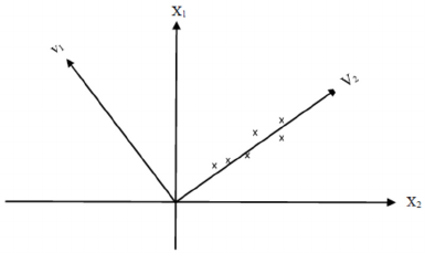
.
Figure 1: Geometric interpretation of SVD method for a
matrix A.
A Modified Fuzzy Lee-Carter Method for Modeling Human Mortality
19
That is, SVD method aims to reorient the coordinate
axes in such a way that these axes follow a more
similar pattern to the points of matrix A. Figure 1
shows the geometric interpretation of the method as
an example. Assuming that matrix A is a
62×
matrix composed of six data points, In Figure 1
these six data points, defined in the coordinate plane
of x
1
-x
2,
can also be expressed in the coordinate
plane of v
1
-v
2
.
To utilize SVD method in equation (6) for
estimating the unknown parameters
0
,
x
c
1
,
x
c and
;
t
f
the following procedure is applied. First,
t
f
’s
are normalized to sum to 0 and
1
x
c ’s to sum to 1.
Then,
0
x
c must equal the average over time of
,
y
x
t
(this follows from the fact that the average value of
t
f
’s is set to 0). Moreover, each
t
f
must equal to
the sum over age of
,0
(y ),
x
tx
c−
since the sum of
1
x
c ’s is set to unity. Then,
1
x
c ’s are estimated by
regressing
,0
(y )
x
tx
c−
on
t
f
without a constant term
separately for each age group x (Lee and Carter,
1992). The spread optimization part of Koissi and
Shapiro’s model which is rewritten as:
minimize
0
0
1
01
||
tT
x
xt
tt
Ts s f
+−
=
+
(7)
subject to:
01 01 ,
00 0
(1 )[ | |] ,
for , 1,..., 1
xxt xxt xt
ccf hssf y
ttt t T
++− + ≥
∀= + + −
(8)
01 01 ,
00 0
(1 )[ | |] ,
for , 1,..., 1
xxt xxt xt
ccf hssf y
ttt t T
+−− + ≤
∀= + + −
(9)
01
,0
xx
ss≥
(10)
Here, the objective is to minimize the total
spreads. Equations (8) and (9) guarantee that each
log-mortality rate
,
Y
x
t
falls within the estimated
ˆ
Y
x
t
at a level h, which is a predetermined small
parameter (Koissi and Shapiro prefer using h = 0).
2.2 Part II: Finding the Model
Parameters
Once the log-mortality rates are fuzzified, the next
step in Koissi and Shapiro’s method is to find
appropriate parameters
A ,
x
B
x
and K
t
for equation
(2). At this point it is worth mentioning that with
multiplication of triangular fuzzy numbers, the
characteristics of the numbers are not preserved
although addition of triangular fuzzy numbers also
results in a triangular fuzzy number. Mesiar (1997)
shows that with weakest triangular norm (T
W
) based
multiplication and addition the shape of the
membership function is preserved for LR-type fuzzy
numbers.
For two symmetric triangular fuzzy numbers
A(,)
A
al=
and B(,),
B
bl=
the shape preserving T
W
-based multiplication and addition are (Koissi and
Shapiro, 2006):
AB( ,max(,))
W
AB
T
ab ll⊕= +
(11)
A B ( , max( | b |, | a |))
W
AB
T
ab l l⊗=
(12)
Using equations (11) and (12), equation (2) can
be rewritten as:
,
Y( , max(,||,||))
xt x x t x x x x t
abk b k
αδβ
=+
(13)
To find the unknown parameters
,
x
a ,
x
b ,
t
k
,
x
α
,
x
β
and
t
δ
; Koissi and Shapiro suggest a
solution to equation (2) by minimizing the total
squared distance between
ABK
WW
xxt
TT
⊕⊗
and
,
Y .
x
t
Here, they make use of Diamond distance as the
fuzzy distance measure. Diamond distance
(Diamond, 1988) between two symmetric triangular
fuzzy numbers
111
A(,)a
α
=
and
222
A(,)a
α
=
is
defined as:
2
12 1 2 1 1
22
22 11 22
(A , A ) ( ) [( )
()][()()]
LR
Daaa
aaa
α
ααα
=− + −
−− + + − +
(14)
Minimizing total Diamond distance leads to
following optimization problem for each age cohort
x and time t:
Minimize
2
,
[A (B K ), Y ]
WW
LR x x t x t
TT
xt
D ⊕⊗
(15)
where
22
,,
,
2
,
2
,,
[A (B K ),Y ] ( )
[max{,||,||}(
)] [ max{ ,| | , | |}
()]
WW
LR x x t x t x x t x t
TT
xxt xxtxt xt
xt x x t x x t x t
xt xt
Dabky
abk b k y
eabk b k
ye
αδβ
αδβ
⊕⊗ =+ −
++ − −
−+++
−+
(16)
FCTA 2015 - 7th International Conference on Fuzzy Computation Theory and Applications
20

This is an unconstrained nonlinear problem as
finding the optimal values of parameters
,
x
a ,
x
b
,
t
k ,
x
α
,
x
β
and
t
δ
require dealing with a maximum
function. Applying SVD,
x
a can be obtained as:
,
1
x
xt
t
ay
T
=
(17)
Finding the parameters
,
x
b ,
t
k ,
x
α
,
x
β
and
t
δ
is less straightforward, because, the structure of
equation (15) does not allow using a derivative
based solution algorithm. Hence, fminsearch tool of
MATLAB optimization application for
unconstrained optimization problems can be utilized
to find the unknown parameters. fminsearch is a
derivative free method for unconstrained nonlinear
optimization problems based on Nelder-Mead
simplex algorithm (Nelder and Mead, 1965).
3 NUMERICAL FINDINGS
The proposed method is applied to mortality data for
Finland. The reason why Finland dataset is selected
for application is that the mortality rates in Finland
show some fluctuations due to some exogenous
effects such as World War II. Furthermore, Koissi
and Shapiro also apply their method on Finland
dataset. In this study, standard LC and the fuzzy LC
models are also applied to the same dataset and the
outcomes are compared with the results obtained
from the proposed method. The data is obtained
freely from “Human Mortality Database” at
www.mortality.org. In all computations total
mortality rates (for both sexes) of seventeen
consecutive five-year-periods 1925-1929, 1930-
1934 …, 2005-2009, and twenty two age cohorts of
[0, 1), [1-5), [5, 10), …, [100, 105) are used (making
374 data points in total).
To demonstrate the results, three example
periods are selected and given in Table 1, 2, and 3.
These tables display the spreads of fuzzified
values of Finland for selected five-year-periods of
1925-1929 (the first time period), 1965-1969 (the
mid-time period in dataset) and 2005-2009 (the last
time period) respectively. The results in these tables
are calculated via Koissi and Shapiro’s fuzzified LC
model (spread
OLS
) and the modified fuzzy LC model
(spread
SVD
).
Tables 1 to 3 illustrate that proposed method give
smaller spreads compared to Koissi and Shapiro’s
method for ten age groups in 1925-1929 period, for
sixteen age groups in 1965-1969 period, and for
twenty age groups in 2005-2009. This shows that the
number of smaller spreads generated during
fuzzification of Y
x,t
by the proposed method are
increasing by time. This trend can be explained by
the advances in accurate data approaches which
result in vagueness reduction, thus smaller spreads.
When the whole dataset is considered, paired t-test
results show that the proposed method is superior to
Koissi and Shapiro’s method in terms of smaller
spread generation (t-value=13.53, p-value=0.000),
smaller absolute distances between observed Y
x,t
and
center values of fuzzified Y
x,t
(t-value=5.07, p-
value=0.000) and smaller squared distances between
observed Y
x,t
and center values of fuzzified Y
x,t
(t-
value=3.88, p-value=0.000) during the fuzzification
of log-mortality rates.
The two methods are also compared in terms of
their
,
Y
x
t
estimations based on the model
parameters obtained from the second parts of the
methods. Figure 2 and 3 illustrate the observed Y
x,t
,
and estimated centers of
,
Y
x
t
with Koissi and
Table 1: Spreads of fuzzified log-mortality values for Finland, 1925-1929.
Age group Spread
OL
S
Spread
SVD
Age group Spread
OL
S
Spread
SVD
[0, 1) 0.3220 0.4419 [50, 55) 0.0750 0.1560
[1, 5) 0.4920 0.3556 [55, 60) 0.1250 0.1533
[5, 10) 0.5300 0.1723 [60, 65) 0.1540 0.1837
[10, 15) 0.4890 0.2333 [65, 70) 0.1860 0.2686
[15, 20) 0.9170 0.4520 [70, 75) 0.1920 0.3123
[20, 25) 1.6470 0.9371 [75, 80) 0.2137 0.2960
[25, 30) 1.3170 0.6741 [80, 85) 0.1970 0.2603
[30, 35) 1.0320 0.4829 [85, 90) 0.2110 0.2300
[35, 40) 0.7380 0.3062 [90, 95) 0.2340 0.2473
[40, 45) 0.3860 0.1300 [95, 100) 0.2340 0.2556
[45, 50) 0.1380 0.1173 [100, 105) 0.3750 0.4252
A Modified Fuzzy Lee-Carter Method for Modeling Human Mortality
21

Table 2: Spreads of fuzzified log-mortality values for Finland, 1965-1969.
Age group Spread
OL
S
Spread
SVD
Age group Spread
OL
S
Spread
SVD
[0, 1) 0.3700 0.3161 [50, 55) 0.0750 0.0931
[1, 5) 0.4923 0.2088 [55, 60) 0.1250 0.1498
[5, 10) 0.5300 0.1304 [60, 65) 0.1540 0.1627
[10, 15) 0.4890 0.1914 [65, 70) 0.1860 0.1847
[15, 20) 0.9170 0.4520 [70, 75) 0.2080 0.2074
[20, 25) 1.6470 0.4548 [75, 80) 0.2194 0.2331
[25, 30) 1.3170 0.3177 [80, 85) 0.1970 0.2184
[30, 35) 1.0320 0.2312 [85, 90) 0.2110 0.2300
[35, 40) 0.7380 0.1385 [90, 95) 0.2340 0.1424
[40, 45) 0.3860 0.1300 [95, 100) 0.2340 0.1717
[45, 50) 0.1380 0.0754 [100, 105) 0.3750 0.1945
Table 3: Spreads of fuzzified log-mortality values for Finland, 2005-2009.
Age group Spread
OL
S
Spread
SVD
Age group Spread
OL
S
Spread
SVD
[0, 1) 0.4180 0.2102 [50, 55) 0.0750 0.0401
[1, 5) 0.4926 0.0852 [55, 60) 0.1250 0.1468
[5, 10) 0.5300 0.0951 [60, 65) 0.1540 0.1450
[10, 15) 0.4890 0.1561 [65, 70) 0.1860 0.1141
[15, 20) 0.9170 0.4520 [70, 75) 0.2240 0.1192
[20, 25) 1.6470 0.0487 [75, 80) 0.2251 0.1801
[25, 30) 1.3170 0.0175 [80, 85) 0.1970 0.1831
[30, 35) 1.0320 0.0194 [85, 90) 0.2110 0.2300
[35, 40) 0.7380 0.0028 [90, 95) 0.2340 0.0542
[40, 45) 0.3860 0.1300 [95, 100) 0.2340 0.1011
[45, 50) 0.1380 0.0401 [100, 105) 0.3750 0.0003
Shapiro’s and modified methods for age groups [5,
10) and [40-45) respectively. These two age groups
are selected randomly as examples. In both figures,
the horizontal axis stand for time periods (1=1925-
1929, …, 17=2005-2009), whereas the vertical axis
depicts the log-mortality rates. The numerical
findings show that the proposed method displays
better similarity between observed and estimated
log-mortality rates compared to Koissi and Shapiro’s
method. In fact, paired t-test results show that the
modified method is superior to Koissi and Shapiro’s
method in terms of smaller spread generation (t-
value=13.97, p-value=0.000), smaller absolute
distances between observed Y
x,t
and center values of
fuzzified Y
x,t
(t-value=2.69, p-value=0.004) and
smaller squared distances between observed Y
x,t
and
center values of fuzzified Y
x,t
(t-value=4.19, p-
value=0.000) in estimating the log-mortality rates.
As depicted in Figure 2 and 3, the proposed
method gives better fits mainly due to the utilization
of SVD in fuzzifying Y
x,t
values. On the other hand,
Koissi and Shapiro make use of OLS, therefore, the
resulting centers of
,
Y
x
t
follows a linear trend which
is incapable of capturing the fluctuations in data.
However, in Finland mortality rates during
World War II are higher compared to the other
periods, thus the data show fluctuations and even
outlier points for some age groups. In contrast to
Koissi and Shapiro’s method, the proposed method
has the ability to reflect data pattern, thus it gives
better fits as the estimation of model parameters
phase utilizes the better fitted
,
Y
x
t
values.
Finally, the standard LC method is applied to the
same dataset as well (although the homoscedasticity
assumption is violated). When the proposed method
is compared with the standard LC method, paired t-
tests on absolute and squared distances between the
observed Y
x,t
and the estimated centers of
,
Y
x
t
show
that standard LC method gives better results than the
modified one (t-value=6.20, p-value=0.004; t-
value=4.09, p-value=0.000 respectively). However,
as mentioned before, standard LC model cannot be
applied in cases where there is vagueness in
assumptions related with the homoscedasticity and
the magnitude of variance of error terms.
In fact, the
standard LC method cannot be used in this data set
as it requires the data in each age group to be
normally distributed with mean 0 and a small
FCTA 2015 - 7th International Conference on Fuzzy Computation Theory and Applications
22
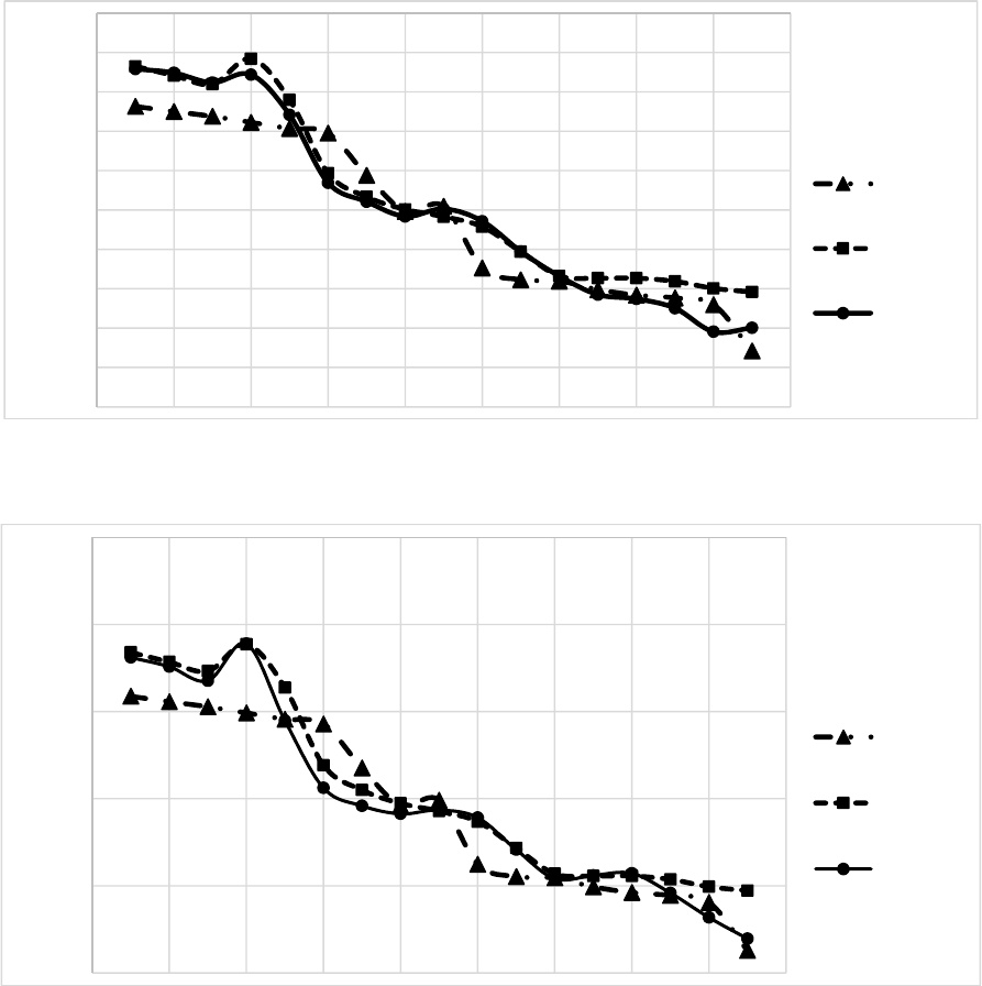
Figure 2: Comparison of observed
,
x
t
Y
and estimated centers of
,
Y
x
t
with Koissi and Shapiro’s and modified methods for
age group [5, 10).
Figure 3: Comparison of observed
,
x
t
Y
and estimated centers of
,
Y
x
t
with Koissi and Shapiro’s and modified methods for
age group [40, 45).
variance
2
ε
σ
. In Finland data set, there are seventeen
data points for each age group separately which do
not a normality test to be performed to see whether
the homoscedasticity assumption is met. Thus, the
better results obtained by standard LC method do
not make sense as the basic assumption of standard
LC approach is violated.
4 CONCLUSIONS
In this paper, a modified version of Koissi and
Shapiro’s fuzzified LC method is proposed. The
proposed method makes use of SVD in fuzzification
of observed log-mortality rates instead of taking
time as the independent variable. Numerical findings
show that proposed method is better in smaller
spread generation and mortality rate estimation even
-10
-9,5
-9
-8,5
-8
-7,5
-7
-6,5
-6
-5,5
-5
024681012141618
log-mortality rate
time period
Yxt-OLS
Yxt-SVD
Yxt-
observed
-6,5
-6
-5,5
-5
-4,5
-4
0 2 4 6 8 10 12 14 16 18
log-mortality rate
time period
Yxt-OLS
Yxt-SVD
Yxt-
observed
A Modified Fuzzy Lee-Carter Method for Modeling Human Mortality
23
the utilized dataset reveal some fluctuations within
time.
The proposed method can be used in cases of
heteroscedasticity and other violations where
standard LC method cannot be applied. In fact the
method gives reasonable estimations when the
number or the quality of data do not permit standard
LC or similar stochastic methods to be used.
The future mortality rates can be forecasted via
estimating future
K
t
values with some suitable
fuzzy time series analysis based on the
K
t
values
obtained from the modified model. As well as this,
the modified fuzzy LC method for estimating
mortality rates can be extended to model fertility and
migration rates. Once the three vital rates (mortality,
fertility, and migration rates) are known it may be
possible to develop a fuzzy population forecasting
model, which may be a research topic of a future
work.
REFERENCES
Ahcan, A., Medved, D., Olivieri, A. and Pitacco, E. (2014)
‘Forecasting mortality for small populations by mixing
mortality data’, Insurance: Mathematics and
Economics, vol. 54, pp. 12–27.
Ahmadi, S. S. and Li, J. S. (2014) ‘Coherent mortality
forecasting with generalized linear models: A
modified time-transformation approach’, Insurance:
Mathematics and Economics, vol. 59, pp. 194–221.
Booth, H. (2006) ‘Demographic forecasting: 1980 to 2005
in review’, International Journal of Forecasting, vol.
22, pp. 547-581.
Brouhns, N., Denuit, M. and Vermunt, J. K. (2002) ‘A
Poisson log-bilinear approach to the construction of
projected life tables’, Insurance: Mathematics &
Economics, vol. 31, no. 3, pp. 373–393.
Chang, Y. H. O. and Ayyub, B. M. (2001) ‘Fuzzy
regression methods – A comparative assessment’,
Fuzzy Sets and Systems, vol. 119, pp. 187–203.
Christiansen, M. C., Niemeyer, A. and Teigiszerová L.
(2015) ‘Modeling and forecasting duration-dependent
mortality rates’, Computational Statistics and Data
Analysis, vol. 83, pp. 65–81.
Currie, I. D., Durban, M. and Eilers, P. H. C. (2004)
‘Smoothing and forecasting mortality rates’, Statistical
Modelling, vol. 4, no. 4, pp. 279–298.
Danesi, I. L., Haberman, S. and Millossovich, P. (2015)
‘Forecasting mortality in subpopulations using Lee–
Carter type models: A comparison’, Insurance:
Mathematics and Economics, vol. 62, pp. 151–161.
De Jong, P and Tickle, L. (2006) ‘Extending Lee-Carter
Mortality Forecasting’, Mathematical Population
Studies, vol. 13, pp. 1-18.
Diamond, P. (1988) ‘Fuzzy least squares’, Information
Sciences, vol. 46, pp. 141-157.
French, D. (2014) ‘International mortality modelling - An
economic perspective’, Economics Letters, vol. 122,
pp. 182–186.
Giacometti, R., Bertocchi, M., Rachev, S. T. and Fabozzi,
F. J. (2012) ‘A comparison of the Lee–Carter model
and AR–ARCH model for forecasting mortality rates’,
Insurance: Mathematics and Economics, vol. 50, pp.
85–93.
Hatzopulos, P. and Haberman, S. (2011) ‘A dynamic
parameterization modeling for the age–period–cohort
mortality’, Insurance: Mathematics and Economics,
vol. 49, pp. 155–174.
Hyndman, R. J. and Ullah, M. S. (2007) ‘Robust
forecasting of mortality and fertility rates: A
functional data approach’, Computational Statistics &
Data Analysis, vol. 51, pp. 4942-4956.
Keyfitz, N. (1988) Applied Mathematical Demography,
New York: John Wiley.
Koissi, M. C. and Shapiro, A. F. (2006) ‘Fuzzy
formulation of Lee-Carter model for mortality
forecasting’, Insurance: Mathematics and Economics,
vol. 39, pp. 287-309.
Lazar, D. and Denuit, M. (2009) ‘A multivariate time
series approach to projected life tables’, Applied
Stochastic Models in Business & Industry, vol. 25 no.
6, pp. 806–823.
Lee, R. D. (2000) ‘The Lee–Carter method for forecasting
mortality, with various extensions and applications’,
North American Actuarial Journal, vol. 1 no. 4, pp.
80–91.
Lee, R. D. and Carter, L. R. (1992) ‘Modelling and
Forecasting US Mortality’, Journal of American
Statistical Association, vol. 87, pp. 659-671.
Lee, R. D. and Tuljapurkar, S. (1994) ‘Stochastic
Population Projections for the U.S.: Beyond High,
Medium and Low’, Journal of the American Statistical
Association, vol. 89 no. 428, pp. 1175-1189.
Li, S. H. and Chan, W. S. (2005) ‘Outlier analysis and
mortality forecasting: The United Kingdom and
Scandinavian countries’ Scandinavian Actuarial
Journal, vol. 3, pp. 187-211.
Lindh, T. (2003) ‘Demography as a forecasting tool’,
Futures, vol. 35, pp. 37-48.
Mandel, J. (1982) ‘Use of the singular value
decomposition in regression analysis’, The American
Statistician, vol. 36, no. 1, pp. 15-24.
Meisar, R. (1997) ‘Shape preserving additions of fuzzy
intervals’, Fuzzy Sets and Systems, vol. 86, pp. 73-78.
Nelder, J. A. and Mead, R. (1965) ‘A Simplex Method for
Function Minimization’, The Computer Journal, vol. 7
no. 4, pp. 308-313.
Renshaw, A. E. and Haberman, S. (2003) ‘Lee–Carter
mortality forecasting with age specific enhancement’,
Insurance: Mathematics and Economics, vol 33, no. 2,
pp. 255–272.
Tanaka, H., Uejima, S. and Asai, K. (1982) ‘Linear
regression analysis with fuzzy model’, IEEE
Transactions on Systems, Man, and Cybernetics:
Systems, vol. 2, pp. 903-907.
FCTA 2015 - 7th International Conference on Fuzzy Computation Theory and Applications
24
