
A Heuristic Solution for Noisy Image Segmentation using Particle Swarm
Optimization and Fuzzy Clustering
Saeed Mirghasemi, Ramesh Rayudu and Mengjie Zhang
School of Engineering and Computer Science, Victoria University of Wellington, Wellington, New Zealand
Keywords:
Noisy Image Segmentation, Fuzzy C-Means, Particle Swarm Optimization, Impulse Noise.
Abstract:
Introducing methods that can work out the problem of noisy image segmentation is necessary for real-world
vision problems. This paper proposes a new computational algorithm for segmentation of gray images contam-
inated with impulse noise. We have used Fuzzy C-Means (FCM) in fusion with Particle Swarm Optimization
(PSO) to define a new similarity metric based on combining different intensity-based neighborhood features.
PSO as a computational search algorithm, looks for an optimum similarity metric, and FCM as a clustering
technique, helps to verify the similarity metric goodness. The proposed method has no parameters to tune, and
works adaptively to eliminate impulsive noise. We have tested our algorithm on different synthetic and real
images, and provided quantitative evaluation to measure effectiveness. The results show that, the method has
promising performance in comparison with other existing methods in cases where images have been corrupted
with a high density noise.
1 INTRODUCTION
The concept of partitioning an image into homo-
geneous regions, usually referred to as image seg-
mentation, is an important mid-level image analy-
sis technique for many high-level afterwards applica-
tions such as object detection (Zhuang et al., 2012;
Ant
´
uNez et al., 2013), image recognition (Ferrari
et al., 2006; Kang et al., 2011), image retrieval (Mei
and Lang, 2014), image compression (Zhang et al.,
2014), and video control/surveillance (Mahalingam
and Mahalakshmi, 2010; Zhang et al., 2009). Since
its emersion in mid 20th century, it has been revolu-
tionized a lot, not only to be applied to more practi-
cal problems, but also to cope with the unstoppable
trend of demand for more accurate detection, classi-
fication, and recognition in a variety of applications.
A small but quite practicable section of image seg-
mentation is devoted to noisy image segmentation in
which fuzzy clustering usually performs as a powerful
tool (Cai et al., 2007). The common fuzzy clustering
algorithm for this matter is Fuzzy C-Means (FCM)
(Hathaway et al., 2000) which due to simplicity and
applicability is one of the most used clustering algo-
rithms. It is also known for better performance in case
of poor contrast, overlapping regions, noise and in-
tensity inhomogeneities (Benaichouche et al., 2013).
The fuzzy membership of FCM allows each datapoint
to belong to every existing cluster with different de-
grees of membership. This is especially of interest in
noisy data clustering where it has been widely used to
cluster noisy contaminated data.
Lots of the so far proposed FCM-based algorithms
for noisy image segmentation are parameter depen-
dent (Ahmed et al., 1999; Szilagyi et al., 2003; Chen
and Zhang, 2004; Cai et al., 2007). Usually, these
parameters make a trade-off between preserving the
details in an image and eliminating the noise which
makes the applicability of these methods limited to
noisy images in which the amount of noise is known.
This means that the best segmentation results are only
obtained when a prior knowledge of the noise volume
is available. Another issue is that they usually fail to
perform well when the image is presented with heavy
impulse noise as a common type of noise mainly be-
cause impulse noises are not easy to deal with.
This paper introduces a heuristic fuzzy algorithm
for noisy image segmentation with no parameters
to tune in advance according to the noise volume.
The utilized features have been specifically chosen to
compensate for impulse noise, and the algorithm has
been designed to confront heavy noise. In this way,
we incorporate spatial, texture, and fuzzy member-
ship values to achieve better results.
The rest of this paper is organized as follows. Sec-
tion 2 is devoted to the research background of this
study. Section 3 describes the proposed method. Ex-
perimental results, datasets, and parameter settings
Mirghasemi, S., Rayudu, R. and Zhang, M..
A Heuristic Solution for Noisy Image Segmentation using Particle Swarm Optimization and Fuzzy Clustering.
In Proceedings of the 7th International Joint Conference on Computational Intelligence (IJCCI 2015) - Volume 1: ECTA, pages 17-27
ISBN: 978-989-758-157-1
Copyright
c
2015 by SCITEPRESS – Science and Technology Publications, Lda. All r ights reserved
17

are presented in section 4, and section 5 is dedicated
to conclusions and future work.
2 BACKGROUND
This section starts with the introduction of the pri-
mary FCM and its variants. We then introduce PSO as
the heuristic algorithm we have utilized in this paper,
and then related work would be presented.
2.1 Fuzzy C-Means Related Algorithms
The Fuzzy C-Means (FCM) as a clustering algorithm
was first introduced in (Dunn, 1973), and then ex-
tended in (Hathaway et al., 2000). The aim in FCM is
to find c partitions via minimizing the following ob-
jective function:
J =
N
∑
i=1
C
∑
j=1
u
m
ji
d
2
(x
i
,v
j
) (1)
where X
X
X =
=
= {x
x
x
1
1
1
,
,
,x
x
x
2
2
2
,
,
,.
.
..
.
..
.
.x
x
x
N
N
N
} is a dataset in which x
i
rep-
resents a p-dimensional array datapoint in R
p
, and N
is the number of datapoints (p is the number of fea-
tures attributed to each datapoint), C is the number
of clusters, u
i j
is the degree of membership of x
x
x
i
i
i
to
cluster j, which meets u
i j
∈ [0,1] and
C
∑
i=1
u
i j
= 1, m
is the degree of fuzziness, v
j
is the prototype of clus-
ter j, and d
2
(x
i
,v
j
) is the distance difference between
datapoint x
x
x
i
i
i
and cluster center v
v
v
j
j
j
. The two following
iterative formulas are necessary but not sufficient for
J to be at its local extrema. u and v get updated using
these equations till termination threshold is satisfied:
v
k
j
=
N
∑
i=1
u
k
ji
m
x
i
N
∑
i=1
u
k
ji
m
(2)
u
k+1
ji
=
1
C
∑
l=1
d
ji
d
li
2/m−1
(3)
Although FCM itself fails at the segmentation of
noisy images, utilizing the basic concept a number
of algorithms have been created to cover this failure
(Ahmed et al., 1999; Chen and Zhang, 2004; Szilagyi
et al., 2003; Cai et al., 2007; Krinidis and Chatzis,
2010). A common approach in this manner (Ahmed
et al., 1999) known as FCM S was introduced in
which FCM objective function is modified to deal
with intensity inhomogeneities posing in segmen-
tation of magnetic resonance images. The new
objective function is as follows:
J =
N
∑
i=1
C
∑
j=1
u
m
ji
d
2
(x
i
,v
j
) +
α
N
R
N
∑
i=1
C
∑
j=1
u
m
ji
∑
r∈N
k
d
2
(x
r
,v
j
)
(4)
where N
k
is the set of neighbors within the neighbor-
ing window around x
i
, N
R
is its cardinality, and x
r
rep-
resents the neighbor of x
i
. How the neighbors are af-
fecting the objective function is controlled by α. The
new updating formulas for u and v are obtained ac-
cording to Lagrange multipliers taking partial deriva-
tives of the new objective function. The new objec-
tive function allows the neighboring pixels to affect
the labeling procedure of a pixel. Then two modifi-
cations of FCM S algorithm were proposed in (Chen
and Zhang, 2004) mainly trying to reduce the com-
putation of FCM S. These two algorithms known as
FCM S1 and FCM S2 use a pre-calculated mean and
median-filtered image of the noisy image as a sub-
stitution for neighbor pixel labeling in each iteration
which results in a faster algorithm. The modified ob-
jective function is:
J =
N
∑
i=1
C
∑
j=1
u
m
ji
d
2
(x
i
,v
j
) + α
C
∑
j=1
∑
r∈N
k
u
m
jr
d
2
(x
r
,v
j
) (5)
where x
r
is the mean or median average of the
neighboring pixels around x
i
.
For even a faster performance, EnFCM was pro-
posed (Szilagyi et al., 2003). Here again, a linearly-
weighted local filter is applied to image in advance
according to:
ξ
i
=
1
1 + α
x
i
+
α
N
R
∑
r∈N
k
x
r
(6)
in which ξ
i
is the gray level value of the pixel i, and
α plays the same role as before. Then the clustering
procedure is performed on the gray-level histogram
obtained from the filtered image. As there are only
256 gray levels in an image, and having in mind that
the number of pixels in an image are generally much
larger than 256, this algorithm is quite fast, and also
has better performance in noisy image segmentation
compared to FCM S. The new objective function is
introduced as:
J =
Q
∑
i=1
C
∑
j=1
γ
i
u
m
ji
d
2
(ξ
i
,v
j
) (7)
where Q denotes the number of gray levels, and ξ
i
is
the number of pixels having a gray value equal to i.
The so far mentioned algorithms, although having
great achievements dealing with noise, they all suf-
fer from a common problem which is the parameter
ECTA 2015 - 7th International Conference on Evolutionary Computation Theory and Applications
18

α. This parameter keeps a trade-off between the vol-
ume of noise and the details of an image. In other
words, it should be large enough to compensate for
noise and should be small enough to preserve details
of an image like edges. That is why the performance
of these algorithms is α-dependent which is a disad-
vantage when dealing with generic image segmenta-
tion. To make up for this, FGFCM was proposed in
(Cai et al., 2007) incorporating local spatial and gray
information. A new filtering factor, S
i j
is proposed
which acts as a local similarity measure:
S
i j
=
e
−max(|p
i
−p
j
|,|q
i
−q
j
|/λ
s
)−||x
i
−x
j
||
2
/λ
g
σ
2
i
, i 6= j
0 i = j
(8)
σ
i
=
v
u
u
t
∑
j∈N
k
k x
i
− x
j
k
2
N
R
(9)
where i stands for the pixels in the center of the sliding
window, and j is one of the neighboring pixels falling
in the neighborhood window, and (p
k
,q
k
) is the coor-
dinates of the pixel k in the neighboring window. λ
s
and λ
g
are parameters with functioning similar to α.
Like EnFCM, FGFCM performs clustering on the ba-
sis of histogram information obtained from the pro-
posed filtering factor. Although FGFCM acts less
parameter-independent introducing λ
s
and λ
g
, again
its performance is influenced by the variation of λ
g
(Krinidis and Chatzis, 2010).
Regardless of the fact that all these methods per-
form reasonably well on noisy image segmentation,
they have parameters that need to be tuned according
to the volume and type of noise. Although λ
s
could
be fixed in 3 according to (Cai et al., 2007), α and λ
g
have to be adjusted empirically. They have to be large
to make up for the noise, and have to be small to keep
the details of an image. This makes the applicabil-
ity of them limited to images with prior information
about the noise and its volume. Therefore, the need
for parameter-free algorithms which can adaptively
be used for noisy image segmentation is essential. In
addition, the existing methods fail to produce accurate
segmentation results when the noise is heavy, which
is another motivation for the proposed method in this
paper.
2.2 Particle Swarm Optimization
Particle Swarm Optimization is a computational op-
timization algorithm introduced in (Eberhart and
Kennedy, 1995; Kennedy and Eberhart, 1995). Due
to efficiency, robustness, and simplicity (Engelbrecht,
2007) the technique has been modified many times,
for general and specific applications. The search al-
gorithm is motivated by the social behaviors of or-
ganisms. Particularly, choreography of birds flock
led to the design of PSO. The algorithm is initial-
ized with a swarm of potential solutions in a mul-
tidimensional space. Each solution, also known as
particle, has the ability to move. Therefore, parti-
cle i has two parameters as x and v which specify
its location and speed in the search space, respec-
tively. During the movement, each particle updates
its position and velocity according to its own expe-
rience, and that of its neighbors. i is in interactive
communication with neighboring particles in order
to find the best position (final solution). The best
so-far position of each particle is called pbest, and
the best so-far position in the whole swarm is called
gbest. What really determines the goodness of pbest,
gbest, and basically all particles is a fitness function
which is an essential part of PSO algorithm. The fit-
ness function specifies the nature of the optimization
problem, and is designed according to the applica-
tion. Briefly, assuming a D-dimensional search space
the ith particle is represented by X
X
X
i
i
i
=
=
= (
(
(x
x
x
i1
,
,
,x
x
x
i2
.
.
..
.
..
.
.x
x
x
iD
)
)
)
and V
V
V
i
i
i
=
=
= (
(
(v
v
v
i1
,
,
,v
v
v
i2
,
,
,.
.
..
.
..
.
.,
,
,v
v
v
iD
)
)
) as D-dimensional arrays
for the positions and velocities. x
x
x and v
v
v are updated
using these two equations:
v
k+1
id
= w ×v
k
id
+c
1
r
1
(pbest
d
−x
k
d
)+c
2
r
2
(gbest
d
−x
k
d
)
(10)
x
k+1
id
= x
k
id
+ v
k+1
id
(11)
where d = 1,2,...,D, i = 1,2,...,N, are the sizes of di-
mension and swarm, c
1
and c
2
are positive constants,
r
1
and r
2
are random numbers, uniformly distributed
in the interval [0,1], k = 1, 2,..., denotes the iteration
number, pbest
d
and gbest
d
represent pbest and gbest
in the dth dimension, and w is inertia weight which
controls the influence of previous velocities on the
new velocity. Larger inertia weights indicate larger
exploration through the search space while smaller
values of the inertia weight restrict the search on a
smaller space (Engelbrecht, 2007). Typically, PSO
starts with a larger w, and the decreases gradually over
the iterations. We have adopted the following equa-
tion for w to simulate its descending property:
w = (w
initial
− w
f inal
) ×
(k
max
− k)
k
max
+ w
f inal
(12)
where w
initial
, is the preliminary value of w, w
f inal
is
the final value of w, k is the iteration number, and k
max
is the maximum number of iterations.
A Heuristic Solution for Noisy Image Segmentation using Particle Swarm Optimization and Fuzzy Clustering
19
2.3 Related Work
A couple of research works have been proposed in an
attempt to combine heuristic algorithms particularly
PSO with FCM. The common approach (Zhang et al.,
2012; Benaichouche et al., 2013; Tran et al., 2014)
is that potential solutions (particles) are possible val-
ues for cluster centers within the intensity diversity of
pixels. They take the objective function of a FCM-
based clustering method as the fitness function, and
then try to find the optimum positions of the clus-
ter centers that minimize the objective function the
most. This will omit the updating formula for cluster
centers, but again, they need the fuzzy membership
updating formula to obtain the value of membership.
That is why these approaches do not really create a
new algorithm, rather they just try to optimize an ex-
isting one. Knowing that, the FCM-based clustering
methods are already computationally optimized, these
approaches fall effective in special cases that the ob-
jective function of an already existing FCM-based al-
gorithm is not simple enough to be completely opti-
mized by its iterative procedure itself. Since the im-
provement is not significant often for such an opti-
mization case, the better performance is achieved by
including other criteria to the existing algorithm (Tran
et al., 2014; Benaichouche et al., 2013).
Another trend in the literature is investigating the
effect of Gaussian noise in noisy image segmenta-
tion. This paper, unlike the common trend, is focused
on impulse noises as another common type of noise
in image processing. Impulse or fat-tail distributed
noise, which sometimes is referred to as salt and pep-
per noise, can be produced by malfunctioning pixels
in camera sensors, faulty memory locations in hard-
ware, analog-to-digital converter errors or bit errors in
a transmission (Bovik, 2005). This means, images are
usually damaged by impulsive noises during acqui-
sition or transmission. It appears as sparsely occur-
ring white and black pixels. Since the corrupted pixel
by impulsive noise contains no information about the
present image, impulse noisy image segmentation is a
challenging issue.
The proposed approach in this paper, unlike the
existing approaches, uses PSO to define a new simi-
larity criterion for FCM in which segregation between
two datapoints (pixels here) happens by combining
different features extracted from a neighboring win-
dow around each pixel. For this, the new measure-
ment criterion not only utilizes gray and spatial in-
formation, but also uses the fuzzy membership value
to achieve a better performance. Our method intro-
duces a new optimization process in which FCM clus-
tering performance on noisy image segmentation gets
improved by modifying the classic Euclidean metric.
This is different from the common trend that uses
PSO for a better initialization of FCM.
3 THE PROPOSED METHOD
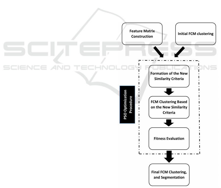
Fig. 1 shows a block diagram of the proposed
method. This figure shows three main steps in
the algorithm: initialization and pre-processing,
PSO search procedure, and final clustering and
segmentation. The general idea is to use PSO to form
a new similarity criterion based on simple texture
properties of a local neighboring window. During the
iterations of the PSO search procedure, FCM will be
used to obtain the parameters related to similarity
measure, and to cluster the noisy data based on
the new similarity criterion. Simply saying, PSO
along with FCM, creates a search space in which the
parameters related to the new similarity measure will
be gradually and automatically optimized.
Figure 1: Block diagram of the proposed method.
ECTA 2015 - 7th International Conference on Evolutionary Computation Theory and Applications
20

3.1 Pre-processing and Initialization
The first step of the proposed algorithm deals with
some initializations and feature construction. The ini-
tialization is carried out via a standard FCM accord-
ing to (2) and (3). This initial clustering provides the
initial cluster centers, V , and the initial membership
values, U, for the PSO procedure in which the new
similarity measurement is formed. This preprocess-
ing not only leads to better segmentation results at the
end, but also builds a deterministic algorithm with sta-
ble outputs.
Feature construction is done in advance for more
simple and efficient implementation. Simple texture
information of a local window around each pixel will
be used to construct the feature matrix. The texture in-
formation is captured by four statistical-based filters
which apply to the intensity values of the pixels in-
side the neighboring window. These sliding-window
filters employ median, variance, standard deviation,
and Wiener filtering.
The Wiener filter (Wiener, 1964) low-pass filters
a grayscale image that has been degraded by ad-
ditive noise. The filter uses a pixel-wise adaptive
Wiener method based on statistics estimated from a
local neighborhood of each pixel. The Wiener filter-
ing is a general way of finding the best reconstruc-
tion of a noisy signal. More specially, it can gener-
ally be applied whenever you have a basis-in-function
space that concentrates “mostly signal” in some com-
ponents relative to “mostly noise” in others. It could
be applied on spatial or wavelet function basis. In spa-
tial (pixel) basis (as utilized in this paper), the Wiener
filter is usually applied to the difference between an
image and its smoothed version. It gives the optimal
way of tapering off the noisy components, so as to
give the best (L
2
norm) reconstruction of the origi-
nal signal. Assuming an observation (noisy image)
(C
i
), which is composed of the original image (S
i
) and
noise (N
i
), we have the measured components as:
C
i
= S
i
+ N
i
(13)
The filter looks for a signal estimator that scales
the individual components of what is measured as:
ˆ
S
i
= C
i
Φ
i
(14)
and finds the signal estimator, Φ
i
, such that it min-
imizes h|
ˆ
S − S|
2
i. Knowing that we are working on
some orthogonal basis, the L
2
norm is just the sum of
squares of the components of what is measured, we
extend the latter, differentiate with respect to Φ
i
, and
set it to zero to obtain:
Φ
is
=
hS
2
i
i
hS
2
i
i + hN
2
i
i
(15)
where hS
2
i
i and hN
2
i
i are estimations of signal and
noise power in each component. Using the estimator
introduced in (Lim, 1990), Wiener estimates the local
mean (ρ), and variance (σ
2
) around each pixel:
ρ =
1
MN
∑
n
1
,n
2
∈η
a(n
1
,n
2
)
σ
2
=
1
MN
∑
n
1
,n
2
∈η
a
2
(n
1
,n
2
) − ρ
2
(16)
where η is the N ×M local neighborhood of each pixel
in the image, and n
1
and n
2
are the coordinates of
pixel a. Then, a pixel-wise Wiener filter using these
estimates is created:
b(n
1
,n
2
) = ρ +
σ
2
− v
2
σ
2
(a(n
1
,n
2
) − ρ) (17)
where v
2
is the noise variance related to the average
of all the local estimated variances.
Although some of the filters for constructing the
feature matrix have been individually used for FCM-
based image segmentation (Chen and Zhang, 2004),
this is the first time that their combination is used
for noisy image segmentation. To be able to com-
bine noise degradation properties of each filter on an
image, we use them all to build a new similarity cri-
terion. This not only allows us to benefit from the
properties of each filter, but also gives our approach
the ability to adaptively come up with a unique solu-
tion for each image.
3.2 A New Similarity Measure
The main contribution of this paper is that it incorpo-
rates simple statistical features of a neighboring win-
dow around each pixel into the distance calculation
metric of the classical FCM using PSO. Motivated by
the texture detection algorithm in (Tian et al., 2013),
we modify d
2
(x
i
,v
j
) in (1) as below:
d
2
(x
i
,v
j
) =k x
i
− v
j
k (1 −
4
∑
p=1
µ
p
F
i j(p)
) (18)
where k x
i
− v
j
k is the Euclidean distance between
the gray (intensity) information of each pixel and jth
cluster center, p is the number of features, and µ
µ
µ
p
p
p
are
the coefficients to be obtained subjected to:
0 < µ
p
< 1 (19a)
4
∑
p=1
µ
p
F
i j(p)
≤ 1 (19b)
A Heuristic Solution for Noisy Image Segmentation using Particle Swarm Optimization and Fuzzy Clustering
21

F
i j
is a fusion of one-at-a-time (one out of four) fea-
ture attributed to each pixel, and some other informa-
tion from the rest of pixels falling inside the neighbor-
ing window as:
F
i j
=
N
R
∑
n=1
u
n
× ( f
n
i
− f
i
) × (e
−|x
n
i
−v
j
|
)
N
R
∑
n=1
( f
n
i
− f
i
) × (e
−|x
n
i
−v
j
|
)
(20)
where n is the index for the pixels within the
neighboring window for the similarity metric (N
R
is the cardinality of neighboring pixels), u is the
fuzzy membership value, f is the considering feature
from the previously-built feature matrix, f
i
is the
corresponding feature value of the pixel x
i
at the
center of the neighboring window for the similarity
metric, x is the intensity values, and v
j
is the cluster
center for cluster j. µ coefficients are determined
and optimized gradually during the PSO procedure to
produce a proper similarity measure that can mitigate
the influence of noise to the greatest extend.
Equation (18) tries to reduce the distance between
a pixel and a cluster center with respect to the
information obtained from the neighboring window
around the pixel. This is not limited to only one
feature though, as (18) indicates. This is due to the
requirement that one feature alone may not be able
to attenuate the effect of noise. Having different
features included in the new similarity measure,
the search procedure provided by PSO enables this
reduction to take the best out of each feature in an
optimizing manner.
In addition, we have no parameters which need
tuning according to the noise volume. In our method,
all the related parameters (except for the neighboring
window sizes) in the similarity criterion get tuned
automatically during the iterations of PSO procedure
according to the noise properties of the test image.
3.3 PSO Representation
Apart from general motivations to utilize PSO for op-
timization problems (mentioned in sub-section 2.2),
simplicity of representing our optimizing problem in
the form of a PSO-based process is another motiva-
tion. The particle representation of PSO suits well
our objectives toward obtaining the optimum weights
for the new similarity measure. Also, the encoding
and decoding procedure is quite straightforward in
our problem. Overall, PSO is utilizes to adaptively
tune all the parameters associated with the new sim-
ilarity measure specifically for each image, based on
the volume of noise and feature properties.
The previously constructed feature matrix, initial
fuzzy membership values and cluster centers are used
as inputs for the PSO optimization procedure. As (18)
and (20) indicate, the new similarity criterion is de-
signed using four features. Associated with each fea-
ture is a µ coefficient. PSO is applied to find the best
contribution of each feature by determining µ values.
Therefore, each particle, p
p
p
i
i
i
, contains potential values
for µ coefficients in form of p
p
p
i
i
i
=
=
= (
(
(µ
µ
µ
1
1
1
,
,
,µ
µ
µ
2
2
2
,
,
,µ
µ
µ
3
3
3
,
,
,µ
µ
µ
4
4
4
)
)
) that
demonstrates a 4-D search space.
The search space, as (19a) suggests, is defined as
the smooth interval (0,1) for each dimension, and is
restricted continuously according to (19b). During
the PSO search, for each proposed combination of
µ values, FCM clustering is performed using (2) and
(3), and then the PSO fitness function is calculated
to evaluate the combination. The fitness function (1)
in which d
2
(x
i
,v
j
) has been substituted by the new
similarity measure as in (18). The best p
p
p
i
i
i
is the parti-
cle that minimizes the fitness function the most. The
fitness function, which basically drives the search al-
gorithm, conveys two important values to the next it-
eration:
1. The best solution that results in the minimum
value of the fitness function.
2. The cluster centers that correspond to that solu-
tion.
When the PSO search finishes, the final combina-
tion of µ values is used for one final clustering. Then,
the pixels will be labeled according to their biggest
membership value to create a segmented image.
One disadvantage of FCM is that it easily gets
trapped in local minima and fails to achieve the
optimum results. To overcome this, the initial four
dimensional array is set to very small positive values.
The inertia factor, w, as a factor to control particle
velocity during the search, has bigger values in the
beginning and smaller values towards the end of the
search. As mentioned in (Mirghasemi et al., 2012),
selecting values between [1,0.5] with the mentioned
updating formula leads to maximum velocity com-
patibility.
3.4 Summary of the Algorithm
Different steps of the proposed method could be sum-
marized as below:
1. Load the noisy image.
2. Build the feature matrix based on Wiener, median,
variance, and standard deviation measures of in-
tensity values in the neighboring window.
ECTA 2015 - 7th International Conference on Evolutionary Computation Theory and Applications
22

3. Set the parameters for FCM clustering, including
the number of clusters.
4. Perform a standard FCM clustering to obtain ini-
tial values for U and V .
5. Initialize PSO with parameters for x, v, iteration
number, particle number, search space dimension
size, and inertia weight.
6. Propose an initial solution for µ
µ
µ values.
7. Form the new similarity measure according to
(18).
8. Perform FCM clustering according to the new
similarity measurement.
9. Evaluate the fitness function: calculate the objec-
tive function of FCM according to (1).
10. Form pbest and gbest according to the fitness
value from step 9.
11. Update x and v according to (11) and (10).
12. Go back to step 6, unless it is the end of iterations.
13. Use the resultant optimized values of
(
(
(µ
µ
µ
1
1
1
,
,
,µ
µ
µ
2
2
2
,
,
,µ
µ
µ
3
3
3
,
,
,µ
µ
µ
4
4
4
)
)
) to do the final similarity measure
calculation and FCM clustering.
14. Use the U matrix for image segmentation.
For a clearer depiction of the proposed algorithm,
the pseudocode is provided for the PSO search pro-
cedure in Algorithm 1. The parameters used in this
pseudocode are as follow: ps, X, V , Pbest, C, k, k
max
,
and w stand for population size, population’s position
matrix, population’s velocity matrix, the population’s
pbest matrix, matrix of population’s corresponding
cluster centres, iteration, iteration number, and iner-
tia weight, respectively.
3.5 Parameter Design
Both PSO and FCM algorithms have intrinsic param-
eters to set. Also, our method has measures for the
sizes of the local neighboring windows in both filter-
ing and new distance forming steps. This sub-section
provides details for all these parameters. As men-
tioned before, parameters related to the new similar-
ity criterion get tuned automatically, and do not need
prior setting. Based on experiments on two different
datasets of gray images, we came up with the parame-
ter adjustment shown in table 1. These parameters are
fixed for every test image of each dataset, and none of
them need to be changed.
Algorithm 1: The PSO search steps.
1: Set the PSO parameters: x, v, k, k
max
, and w; x is
initially [0.001,0.001,0.001,0.001]
2: Set particle one as gbest;
3: k = 0;
4: while k < k
max
do
5: Update w using(12);
6: for each particle i ∈ pi do
7: Form the new similarity metric according to
(18);
8: Perform FCM based on the new similarity met-
ric;
9: Evaluate f (x) according to (1);
10: end for
11: if k = 0 then
12: pbest = f (x);
13: gbest = min(Pbest);
14: c = C(gbest);
15: else
16: pbest = f (x) < pbest;
17: gbest = min(Pbest);
18: c = C(gbest);
19: Update V using (10) and restrict its growth;
20: Update X using (11) and restrict its growth;
21: k = k + 1;
22: end if
23: end while
24: Return gbest and c;
Table 1: Parameter Setting.
Parameter Value
Neighboring window for filtering 5 ×5
Neighboring window for similarity criterion 5 × 5
Weighting exponent (m) 2
Termination threshold for FCM 0.001
Maximum number of iterations for FCM 100
Population size (ps) 20
Iteration number 50
The initial value of the first solution 0.001
c
1
and c
2
in (10) 1
w
initial
and w
f inal
in (12) 1 and 0.5
4 EXPERIMENTAL RESULTS
AND ANALYSIS
In this section, we compare the robustness of our
method in heavy impulse noisy image segmentation
against four other methods. The first one is the hard
clustering method K-means, and the other three are
fuzzy clustering methods named as FCM (Hathaway
et al., 2000), EnFCM (Szilagyi et al., 2003), and
FGFCM (Cai et al., 2007). EnFCM needs tuning for
α, and FGFCM needs tuning for λ
g
according to the
type and volume of noise. We take α = 1.8, λ
s
= 3,
and λ
g
= 6 by investigating the interval [0.5,6] for λ
g
,
A Heuristic Solution for Noisy Image Segmentation using Particle Swarm Optimization and Fuzzy Clustering
23
(a)
(b)
(c)
(d)
(e)
(f)
(g)
S1 S2 S3 S4 S5
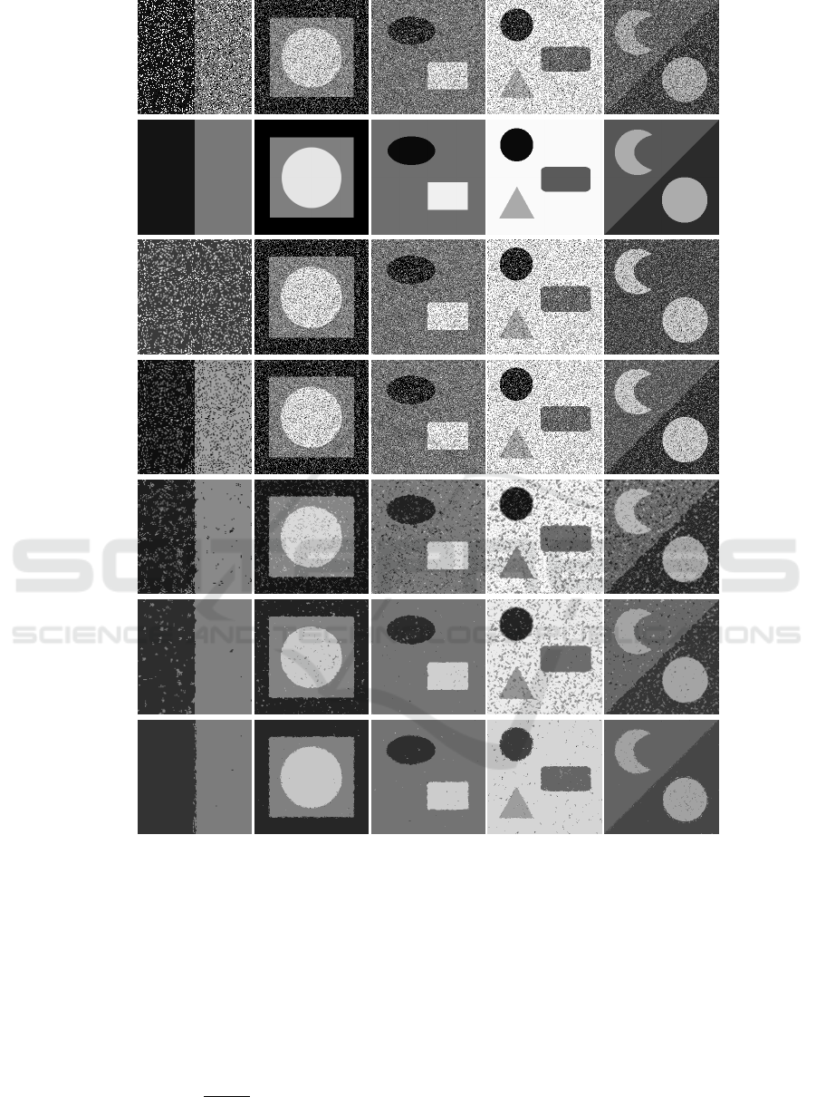
Figure 2: The segmentation results of the proposed algorithm on some sample synthetic images. Rows (a) through (g) are
the noisy corrupted images, the ground truths, K-means, FCM, EnFCM, FGFCM, and our methods segmentation results,
respectively.
and the interval [0.2,8] for α which, according to our
experiments comes with the best performance of En-
FCM and FGFCM methods. To carry out quantita-
tive evaluation, we choose the Segmentation Accu-
racy (SA) introduced in (Ahmed et al., 1999):
SA =
C
∑
i=1
A
i
∩ S
i
C
∑
j=1
S
j
(21)
in which A
i
represents the number of segmented
pixels from the ith cluster and, S
i
is the number of
pixels belonging to the cluster i in the ground truth
image.
To evaluate our method from different perspec-
tives, we have utilized two different datasets. The
first dataset is composed of synthetic images in which
the tested images are 256 × 256 pixels, except for the
image S1 in Fig. 2 which is 128 × 128 pixels. The
ECTA 2015 - 7th International Conference on Evolutionary Computation Theory and Applications
24
(a)
(b)
(c)
(d)
(e)
(f)
(g)
(h)
B1 B2 B3 B4 B5 B6
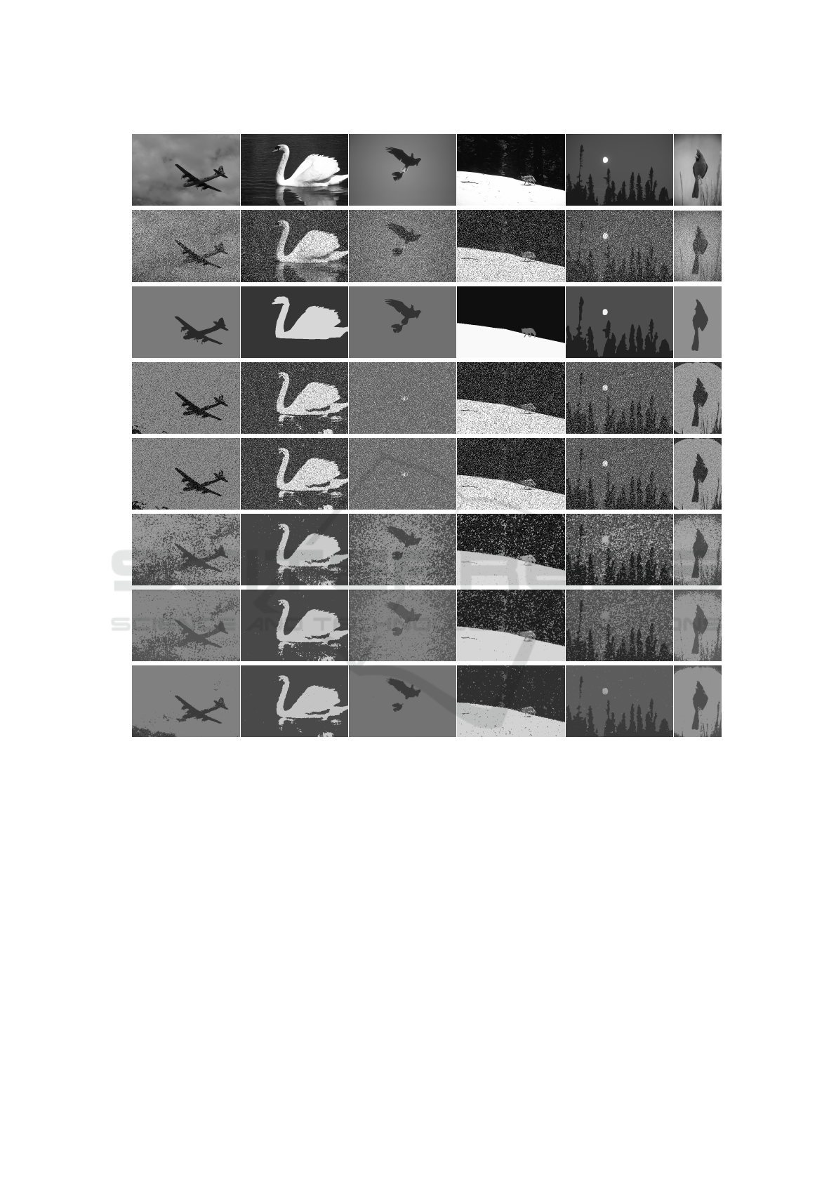
Figure 3: Segmentation results on Berkeley dataset. Rows (a) through (h) are the original images, the noisy corrupted images,
the ground truths, K-means, FCM, EnFCM, FGFCM, and our methods segmentation results, respectively.
second database is the Berkeley image segmentation
(Martin et al., 2001) which is composed of two
sets of images, namely BSDS300 and BSDS500.
These datasets are specifically created for image
segmentation and boundary detection, providing
ground truth for each image. Here, the images are
481 × 321 pixels.
Salt and pepper noise with heavy density of 30%
has been applied through all the testing procedure.
The time performance of our method varies depend-
ing on the image size and its complexity. FCM needs
various numbers of iterations for different images
to satisfy the specified termination threshold. On
average, for images of 256 × 256, on a Intel(R)
Core(TM) i7-4790 CPU @ 3.60GHz machine with
8GB of RAM, it takes 25 minutes for an image to get
processed.
Fig. 2 shows the segmentation results of some
sample synthetic noisy images where the proposed
method performs better in the segmentation of impor-
tant regions. The numbers of specified clusters are 2,
3, 3, 4, and 3 for S1 through S5 images, respectively.
Table 2 also shows the SA metric evaluation of the re-
A Heuristic Solution for Noisy Image Segmentation using Particle Swarm Optimization and Fuzzy Clustering
25

Table 3: Quantitative comparison for Fig. 3, according to the SA metric. Bold numbers indicate the best performance for
each image.
Algorithm B1 B2 B3 B4 B5 B6
K-means 85.3580 86.8103 19.6629 82.9203 70.9614 79.1877
FCM 85.0750 86.8103 19.6629 81.7412 70.9614 79.1877
EnFCM 67.2460 96.5247 58.7644 84.7205 65.4835 73.2668
FGFCM 79.4635 97.3976 66.8882 85.1418 67.2698 79.4748
Our method 96.3309 97.8440 98.8243 97.3401 95.2972 88.4101
Table 2: Quantitative comparison for Fig. 2, according to
the SA metric. Bold numbers indicate the best performance
for each image.
Algorithm S1 S2 S3 S4 S5
K-means 50.0585 84.8183 72.6301 82.7271 52.3180
FCM 85.0676 84.8183 72.6301 82.7271 78.6958
EnFCM 93.0931 95.3562 92.0351 75.4330 79.8469
FGFCM 97.3660 98.2033 99.1229 81.2957 89.4574
Our method 99.3301 98.9701 99.2961 98.2316 97.0128
sults in Fig. 2 on all five methods with bold numbers
representing the best performance for each test im-
age. This table shows that the proposed method per-
forms significantly better than K-means, FCM, and
EnFCM. When it comes to FGFCM, our method still
performs visibly better on S1, S2, S4, and S5. To see
the segmentation difference of FGFCM and the pro-
posed method on image S3, one might need to have
a closer look to see the better performance of our
method. Qualitative evaluation also confirms better
segmentation results obtained by our method. Only
FGFCM has close performance to our method spe-
cially on image S3.
Testing our method with the second database
comes with the segmentation results shown in Fig.
3. Here, six sample images named as B1-B6 are se-
lected. The number of clusters has been set to two
for the fuzzy clustering part in all of them except for
B4 and B5 in which the number of clusters is three.
Again, the proposed method performs both qualita-
tively and quantitatively better than the other four
methods. Although FGFCM has somewhat compara-
ble segmentation results with our method on synthetic
images, Fig. 3 shows that the performance difference
of the proposed method in real images is even greater.
Our method performs better in the segmentation of the
most compact regions. Table 3 provides the SA metric
evaluation of the segmented images shown in Fig. 3.
According to this table, the method that has close per-
formance to our method is not merely FGFCM. Sur-
prisingly, FCM has the second best performance in
B5, and also a close performance to FGFCM in B6.
5 CONCLUSIONS AND FUTURE
WORK
A noisy image segmentation method was proposed
using PSO and FCM. The main objectives were to in-
troduce a new algorithm that is parameter free, has
good performance on impulse noises, and can deal
with heavy density noise. In this way, modifying the
traditional Euclidean similarity measure in FCM us-
ing different intensity-based features extracted from a
neighboring window around each pixel was the main
objective. PSO was utilized to produce an optimum
combination of these features, and FCM was used to
deal with the clustering problem. Spatial, intensity,
and fuzzy criteria are considered in the new similar-
ity metric simultaneously for better performance. The
proposed method introduces a new algorithm to com-
bine different features extracted from the local neigh-
boring window. This puts forward a new way to fuse
features of different types. A future work in this man-
ner is to use more effective features extracted form
the neighboring window. Features than can extend the
applicability of the proposed method to other types of
noises as well. The qualitative and quantitative eval-
uation showed better performances compared with a
few state-of-the-art methods.
REFERENCES
Ahmed, M., Yamany, S., Mohamed, N., and Farag, A.
(1999). A Modified Fuzzy C-Means Algorithm for
MRI Bias Field Estimation and Adaptive Segmenta-
tion. In Taylor, C. and Colchester, A., editors, Med-
ical Image Computing and Computer-Assisted Inter-
vention – MICCAI’99, volume 1679 of Lecture Notes
in Computer Science, pages 72–81. Springer Berlin
Heidelberg.
Ant
´
uNez, E., Marfil, R., Bandera, J. P., and Bandera, A.
(2013). Part-based object detection into a hierarchy of
image segmentations combining color and topology.
Pattern Recogn. Lett., 34(7):744–753.
Benaichouche, A., Oulhadj, H., and Siarry, P. (2013). Im-
proved spatial fuzzy c-means clustering for image
ECTA 2015 - 7th International Conference on Evolutionary Computation Theory and Applications
26

segmentation using {PSO} initialization, mahalanobis
distance and post-segmentation correction. Digital
Signal Processing, 23(5):1390 – 1400.
Bovik, A. C. (2005). Handbook of Image and Video Pro-
cessing (Communications, Networking and Multime-
dia). Academic Press, Inc., Orlando, FL, USA.
Cai, W., Chen, S., and Zhang, D. (2007). Fast and ro-
bust fuzzy c-means clustering algorithms incorporat-
ing local information for image segmentation. Pattern
Recognition, 40(3):825–838.
Chen, S. and Zhang, D. (2004). Robust image segmenta-
tion using fcm with spatial constraints based on new
kernel-induced distance measure. Systems, Man, and
Cybernetics, Part B: Cybernetics, IEEE Transactions
on, 34(4):1907–1916.
Dunn, J. C. (1973). A Fuzzy Relative of the ISODATA Pro-
cess and Its Use in Detecting Compact Well-Separated
Clusters. Journal of Cybernetics, 3(3):32–57.
Eberhart, R. and Kennedy, J. (1995). A new optimizer using
particle swarm theory. In Micro Machine and Human
Science, 1995. MHS ’95., Proceedings of the Sixth In-
ternational Symposium on.
Engelbrecht, A. P. (2007). Computational Intelligence: An
Introduction. Wiley Publishing, 2nd edition.
Ferrari, V., Tuytelaars, T., and Van Gool, L. (2006). Simul-
taneous Object Recognition and Segmentation by Im-
age Exploration. In Ponce, J., Hebert, M., Schmid, C.,
and Zisserman, A., editors, Toward Category-Level
Object Recognition, volume 4170 of Lecture Notes
in Computer Science, pages 145–169. Springer Berlin
Heidelberg.
Hathaway, R., Bezdek, J., and Hu, Y. (2000). Gener-
alized fuzzy c-means clustering strategies using lp
norm distances. Fuzzy Systems, IEEE Transactions
on, 8(5):576–582.
Kang, Y., Yamaguchi, K., Naito, T., and Ninomiya, Y.
(2011). Multiband image segmentation and object
recognition for understanding road scenes. Intelli-
gent Transportation Systems, IEEE Transactions on,
12(4):1423–1433.
Kennedy, J. and Eberhart, R. (1995). Particle swarm op-
timization. In Neural Networks, 1995. Proceedings.,
IEEE International Conference on, volume 4, pages
1942–1948 vol.4.
Krinidis, S. and Chatzis, V. (2010). A robust fuzzy local in-
formation c-means clustering algorithm. Image Pro-
cessing, IEEE Transactions on, 19(5):1328–1337.
Lim, J. S. (1990). Two-dimensional Signal and Image Pro-
cessing. Prentice-Hall, Inc., Upper Saddle River, NJ,
USA.
Mahalingam, T. and Mahalakshmi, M. (2010). Vision based
moving object tracking through enhanced color image
segmentation using haar classifiers. In Proceedings
of the 2nd International Conference on Trendz in In-
formation Sciences and Computing, TISC-2010, pages
253–260.
Martin, D., Fowlkes, C., Tal, D., and Malik, J. (2001).
A database of human segmented natural images and
its application to evaluating segmentation algorithms
and measuring ecological statistics. In Proc. 8th Int’l
Conf. Computer Vision, volume 2, pages 416–423.
Mei, X. and Lang, L. (2014). An image retrieval algorithm
based on region segmentation. Applied Mechanics
and Materials, 596:337341. cited By 0.
Mirghasemi, S., Sadoghi Yazdi, H., and Lotfizad, M.
(2012). A target-based color space for sea target de-
tection. Applied Intelligence, 36(4):960–978.
Szilagyi, L., Benyo, Z., Szilagyi, S., and Adam, H. (2003).
Mr brain image segmentation using an enhanced fuzzy
c-means algorithm. In Engineering in Medicine and
Biology Society, 2003. Proceedings of the 25th An-
nual International Conference of the IEEE, volume 1,
pages 724–726 Vol.1.
Tian, X., Jiao, L., and Zhang, X. (2013). A clustering al-
gorithm with optimized multiscale spatial texture in-
formation: application to SAR image segmentation.
International Journal of Remote Sensing, 34(4):1111–
1126.
Tran, D., Wu, Z., and Tran, V. (2014). Fast Generalized
Fuzzy C-means Using Particle Swarm Optimization
for Image Segmentation. In Loo, C., Yap, K., Wong,
K., Teoh, A., and Huang, K., editors, Neural Infor-
mation Processing, volume 8835 of Lecture Notes in
Computer Science, pages 263–270. Springer Interna-
tional Publishing.
Wiener, N. (1964). Extrapolation, Interpolation, and
Smoothing of Stationary Time Series. The MIT Press.
Zhang, J.-Y., Zhang, W., Yang, Z.-W., and Tian, G. (2014).
A novel algorithm for fast compression and recon-
struction of infrared thermographic sequence based on
image segmentation. Infrared Physics & Technology,
67(0):296–305.
Zhang, Q., Huang, C., Li, C., Yang, L., and Wang, W.
(2012). Ultrasound image segmentation based on
multi-scale fuzzy c-means and particle swarm opti-
mization. In Information Science and Control Engi-
neering 2012 (ICISCE 2012), IET International Con-
ference on, pages 1–5.
Zhang, Q., Kamata, S., and Zhang, J. (2009). Face detection
and tracking in color images using color centroids seg-
mentation. In Robotics and Biomimetics, 2008. RO-
BIO 2008. IEEE International Conference on, pages
1008–1013.
Zhuang, H., Low, K.-S., and Yau, W.-Y. (2012). Multichan-
nel pulse-coupled-neural-network-based color image
segmentation for object detection. Industrial Elec-
tronics, IEEE Transactions on, 59(8):3299–3308.
A Heuristic Solution for Noisy Image Segmentation using Particle Swarm Optimization and Fuzzy Clustering
27
