Predicting Flight Departure Delay at Porto Airport: A Preliminary Study
Hugo Alonso
1,2
and Ant´onio Loureiro
3
1
Universidade de Aveiro, Campus Universit´ario de Santiago, 3810-193 Aveiro, Portugal
2
Universidade Lus´ofona do Porto, Rua Augusto Rosa, 24, 4000-098 Porto, Portugal
3
Aeroporto do Porto, 4470-558 Maia, Portugal
Keywords:
Flight Delay Prediction, Ordinal Classification, Unimodal Model, Neural Networks, Trees.
Abstract:
Managing an airport is very complex. Decisions are often based on common sense and influence several
variables, such as flight delay. This paper considers the problem of predicting flight departure delay at Porto
Airport. As far as we know, this the first study on the subject. The problem is treated as an ordinal classification
task and a suitable approach, based on the so-called unimodal model, isused to predict the delay. The unimodal
model is implemented using neural networks and, for comparison purposes, also using trees.
1 INTRODUCTION
The decisions taken in the management of an airport
are often based on common sense and influence sev-
eral variables, such as flight delay. Reducing this de-
lay presents the advantage of decreasing costs and
increasing the quality of the service provided to the
passengers. It is thus important to find which vari-
ables influence flight delay and use them to predict
it. In this context, several studies, such as (Rebollo
and Balakrishnan, 2014; Wong and Tsai, 2012; Tu
et al., 2008), were carried out and tried to answer the
challenge. For instance, all studies agree that there
is a close relation between arrival delay and depar-
ture delay. Some of them treat flight delay prediction
as a regression problem, predicting the delay by the
minute, and others as a classification problem, pre-
dicting a time interval where the delay will fall.
The problem here considered is to predict flight
departure delay at Porto Airport. As far as we know,
this is the first study on the subject. Given informa-
tion about a flight that will departure from this airport,
such as its arrival delay, we are interested in predict-
ing in which of the following intervals the departure
delay will fall: ] − ∞,0], ]0,15], ]15,30], ]30,60] and
]60,+ ∞[ minutes. Since these intervals can be viewed
as naturally ordered classes, the prediction problem
can be treated as an ordinal classification task. Hence,
we apply a suitable classification method, based on
the so-called unimodal model (Pinto da Costa et al.,
2008), that takes into account the order relation be-
tween the classes, to predict the departure delay class.
The main idea behind this method is that the random
variable class associated with a given query should
follow a unimodal distribution. In order to illustrate
this idea, suppose that, for a certain flight with a given
set of characteristics, the most likely is to observe the
departure delay in the interval ]30, 60] minutes. Given
that there is an order relation between the considered
departure delay intervals, ]15, 30] and ]60,+ ∞[ min-
utes are closer to ]30,60] minutes, and, therefore, the
second most likely interval should be one of these
two. Note that this makes more sense than having,
for instance, the interval ] − ∞,0] minutes for second
most likely. More generally, the probabilities should
decrease monotonically to the left and to the right of
the interval or class where the maximum probability
is attained, i.e., the distribution should be unimodal.
The studies we know where flight delay prediction is
treated as a classification problem either consider two
classes or when they consider more than two classes
they ignore the order relation between them.
The unimodal model can be implemented using
any appropriate machine learning paradigm. Here, we
implement it using neural networks (Haykin, 2009).
Moreover, we measure the importance of the predic-
tor variables by applying a sensitivity analysis pro-
posed in (Kewley et al., 2000) and select the most sig-
nificant for departure delay prediction. For compari-
son purposes, we also implement the unimodal model
using trees (Hastie et al., 2009).
The remainder of this paper is organized as fol-
lows. Section 2 presents the data used in this study.
The unimodal model and the way we apply it to pre-
Alonso, H. and Loureiro, A..
Predicting Flight Departure Delay at Porto Airport: A Preliminary Study.
In Proceedings of the 7th International Joint Conference on Computational Intelligence (IJCCI 2015) - Volume 3: NCTA, pages 93-98
ISBN: 978-989-758-157-1
Copyright
c
 2015 by SCITEPRESS – Science and Technology Publications, Lda. All rights reserved
93

dict flight departure delay are described in Section 3.
The results of our computer experiments are shown
in Section 4 and the conclusions and future work are
given in Section 5.
2 DATA
We had access to a large dataset of 26189 regular
commercial passenger flights performed during 2012.
First, we randomly chose 2619 flights, i.e., about 10%
of all cases, to form a smaller dataset on which we
could carry out our computer experiments in an ac-
ceptable amount of time. Then, we partitioned the
smaller set into training and test subsets. The former
was used to fit models and was assigned 2/3 of the
data, i.e., 1746 cases, while the latter was used to test
selected models and was assigned the remaining 1/3
of the data, i.e., 873 cases.
The target variable in our dataset is the departure
delay interval or class. For reasons that will become
clear later on, we coded the classes using 0 to repre-
sent ]−∞,0], 1 to ]0,15], 2 to ]15,30], 3 to ]30, 60] and
4 to ]60,+∞[ minutes. The class distribution is unbal-
anced, as shown in Figure 1 for the training data. In
fact, classes 0 and 1 are much more frequent than the
others and together they represent almost 80% of the
cases. These two classes together correspond to the
time interval ] − ∞,15] minutes and when the flight
delay falls in this interval it is said at the airport that
there is no commercial delay.
0 1 2 3 4
0
5
10
15
20
25
30
35
40
45
50
Departure delay class
Relative frequency
Figure 1: Relative frequency distribution of the departure
delay class in the training set.
The predictor variables in our dataset are the fol-
lowing:
• arrival delay (in minutes);
• origin and destination of the flight;
• predicted weekday, hour, day and month of the
flight;
• meteorological conditions;
• airline;
• aircraft type;
• aircraft parking stand, ground operation time (in
minutes) and take-off runway.
We chose these predictor variables based on a lit-
erature review regarding departure delay prediction
at other airports and on the experience of the sec-
ond author (an operations manager at Porto Airport
since 2001 and operations worker at this airport since
1987). Several predictor variables took non numerical
values and we had to transform them so that we could
use neural networks. We proceeded as explained next.
The origin and destination of the flight are airports,
which we identified by their coordinates, latitude and
longitude (in degrees), in the World Geodetic System
WGS 84, used by the Global Positioning System (El-
Rabbany, 2006). For the predicted weekday of the
flight, we took 1 to represent Sunday, 2 to Monday,
and so on, until 7 to Saturday. The variable meteo-
rological conditions is binary and we used 0 for nor-
mal visibility operations and 1 for low visibility oper-
ations. The airline was represented by the IATA ac-
counting code; see http://www.iata.org. Finally, the
aircraft type was identified by the aircraft length (in
meters). We did this because we found that different
types have different lengths and that each type, with
three exceptions, has a unique length. In each of the
three exceptions, we took the average of the corre-
sponding lengths, which are close to each other, to
identify the type.
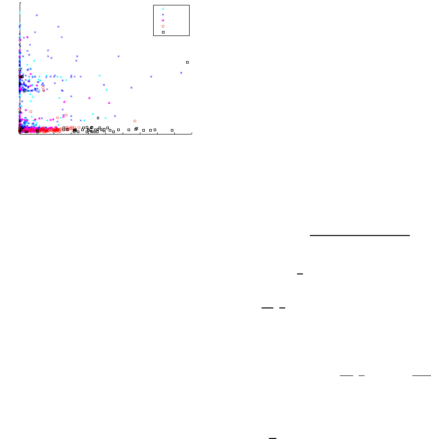
Figure 2 shows a scatter plot of the arrival delay
and ground operation time training data grouped by
the departure delay class. These two predictor vari-
ables are the most significant for departure delay pre-
diction in our implementations of the unimodal model
described next.
3 THE UNIMODAL MODEL AND
ITS APPLICATION TO FLIGHT
DEPARTURE DELAY
PREDICTION
The unimodal model is a machine learning paradigm
intended for supervised classification problems where
the classes are ordered. It was introduced in (Pinto da
Costa et al., 2008) and, for instance, recently applied
in (Fern´andez-Navarro et al., 2015). The main idea
behind this model is that the random variable class
associated with a given query should follow a uni-
modal distribution, so that the order relation between
NCTA 2015 - 7th International Conference on Neural Computation Theory and Applications
94

0 20 40 60 80 100 120 140 160 180 200
0
200
400
600
800
1000
1200
Arrival delay (in minutes)
Ground operation time (in minutes)
Class 0
Class 1
Class 2
Class 3
Class 4
Figure 2: Scatter plot of the arrival delay and ground op-
eration time training data grouped by the departure delay
class.
the classes is respected. In this context, the output
of a classifier where the a posteriori class probabil-
ities are estimated is obliged to be unimodal, i.e., to
have only one local maximum. There are different
ways to impose unimodality and in (Pinto da Costa
et al., 2008) the authors suggested two approaches. In
the parametric approach, a unimodal discrete distribu-
tion, like the binomial and Poisson’s, is assumed and
its parameters are estimated by the classifier. In the
non-parametric approach, no distribution is assumed
and the classifier is trained so that its output becomes
unimodal. In all practical experiments conducted by
the authors, the parametric approach led to better re-
sults, in particular when the binomial distribution was
considered. The superior performance achieved with
this distribution was also justified in theoretical terms.
For these reasons, our focus here is on the binomial
model. Furthermore, since the classifier chosen by us
is a neural network (Haykin, 2009), we refer hereafter
to a binomial network. Its description applied to our
problem is given next.
As mentioned before, given information about a
flight that will departure from Porto Airport, we are
interested in predicting in which of the following in-
tervals the departure delay will fall: ] − ∞,0], ]0, 15],
]15,30], ]30,60] and ]60,+∞[ minutes. Representing
the information given about the flight by x and the
K = 5 departure delay classes ] − ∞,0], ... , ]60,+∞[
minutes by C
1
, ... , C
K
, respectively, Bayes decision
theory (Hastie et al., 2009) suggests classifying the
flight departure delay in the class maximising the a
posteriori probability P(C
k
|x). To that end, the a
posteriori probabilities P(C
1
|x),.. .,P(C
K
|x) need to
be estimated. In the binomial network, these prob-
abilities are calculated from the binomial distribution
B(K−1, p). As this distribution takes values in the set
{0, 1,. .., K − 1}, we take value 0 to represent class
C
1
, 1 toC
2
, and so on, until K − 1 to C
K
. This explains
the coding of the classes presented in the previous
section. Now, since K is known, the only unknown
parameter is the probability of success p. Hence, we
consider a network architecture as in Figure 3 and
train it to adjust all connection weights from layer 1
to layer 3. Note that the connections from layer 3 to
layer 4 have a fixed weight equal to 1 and serve only
to forward the value of p to the output layer of the net-
work where the probabilities from the binomial distri-
bution are calculated. For a given query x, the output
of layer 3 will be a single numerical value in [0,1],
denoted by p
x
. Then, the probabilities in layer 4 are
calculated from the binomial distribution:
P(C
k
|x) = B
k−1
(K − 1, p
x
), k = 1,. .. ,K, (1)
where
B
k−1
(K − 1, p
x
) =
(K − 1)!p
k−1
x
(1− p
x
)
K−k
(k− 1)!(K − k)!
. (2)
When p
x
is in [0,
1
K
[, the highest a posteriori proba-
bility is P(C
1
|x), and, therefore, the predicted flight
departure delay class is C
1
. More generally, when
p
x
is in [
i−1
K
,
i
K
[, for some i in {1, ... , K}, the high-
est a posteriori probability is P(C
i
|x), and, there-
fore, the predicted flight departure delay class is C
i
.
Hence, in order to train the network on a training set
T = {(x
n
,C
x
n
)}
N
n=1
⊂ X × {C
k
}
K
k=1
, where X is the
feature space, we replace C
k
by the value of p corre-
sponding to the midpoint of [
k−1
K
,
k
K
[, i.e., p
k
=
k−0.5
K
,
and apply a suitable optimization algorithm, like the
Marquardt method (Rao, 2009), to find connection
weights that minimise the mean squared error
1
N
N
∑
n=1

p
target
x
n
− p
network
x
n
(w)

2
, (3)
where p
target
x
n
is the value of p replacing C
x
n
and
p
network
x
n
(w) is the output of layer 3 given the query
x
n
and having the network the weights w. In the fol-
lowing, we describe how we apply in our case a sen-
sitivity analysis proposed in (Kewley et al., 2000) to
measure the importance of the predictor variables in a
trained network.
The binomial network, once trained, can be used
to predict a departure delay class
ˆ
C
x
for a particu-
lar flight, based on some information x given about
that flight. Now, recall that each class is represented
by a value in the set {0, 1,... , K − 1} and note that
the value corresponding to
ˆ
C
x
is ˆy
x
= ⌊Kp
x
⌋, where
Predicting Flight Departure Delay at Porto Airport: A Preliminary Study
95

Figure 3: Binomial network for flight departure delay prediction.
p
x
is the output of layer 3 given x. In this context,
let ˆy
j1
, ... , ˆy
jN
denote the values we get by varying
the j-th predictor variable x
j
through its values in the
training set, x
j1
, ... , x
jN
, and holding all other pre-
dictors at their modes (for those that are nominal vari-
ables) or averages (for the remaining). Then, the vari-
ance
V
j
=
1
N − 1
N
∑
n=1
( ˆy
jn
−
ˆy
j
)
2
, (4)
with
ˆy
j
=
1
N
N
∑
n=1
ˆy
jn
, (5)
should be high if x
j
is relevant. Thus, we can measure
the relative importance of the j-th predictor variable
x
j
to the binomial network by
R
j
=
V
j
∑
J
ℓ=1
V
ℓ
× 100%, (6)
where J is the total number of predictors.
Before presenting the results of our computer ex-
periments in the next section, we explain how we se-
lect the predictor variables in the binomial network
and the number of neurons in layer 2. In the beginning
of a first step, all predictor variables available are con-
sidered. The number of neuronsin layer 2 is chosen in
order to minimise the estimate of the prediction error
obtained by applying 10-fold cross-validation to the
training set (Hastie et al., 2009). The measure of error
is the same that is used for training (see (3)). Then, a
network with the variables considered and the number
of neurons selected is trained in the entire training set.
Finally, the importance of the variables to the trained
network are calculated using (6). In the beginning of
the next step, only those predictor variables with an
importance greater than the minimum observed in the
previous step are considered. Everything else is done
in the same way as in the previous step. We repeat this
procedure until there is only one predictor variable to
consider. In the end, we select the binomial network
trained in the entire training set whose predictor vari-
ables and number of neurons in layer 2 are associated
with the least estimate of the prediction error among
all minimum estimates obtained in the various steps.
4 RESULTS
We applied the procedure described in the previous
section to find the best binomial network for depar-
ture delay prediction at Porto Airport. The network
we found through our computer experiments has two
predictor variables and two neurons in layer 2. The
two predictor variables are the ground operation time
and the arrival delay. The first one has an importance
of 50.35% and the second one of 49.65%. Hence,
these two variables are roughly equally important for
the binomial network to predict departure delay. We
applied this network to the test data and the resulting
confusion matrix was the one shown in Table 1.
For comparison purposes, we also implemented
the binomial model using trees (Hastie et al., 2009).
The best pruned tree we found, with the best esti-
mate of the prediction error obtained by applying 10-
fold cross-validation to the training set (Hastie et al.,
2009), has four predictor variables and thirteen ter-
minal nodes. Two of the four predictor variables, the
NCTA 2015 - 7th International Conference on Neural Computation Theory and Applications
96

Table 1: Confusion matrix for the binomial network applied
to the test data.
Predicted class
0 1 2 3 4
True class
0 0 239 0 0 0
1 0 421 8 1 0
2
0 76 27 8 0
3 0 22 9 37 0
4
0 8 1 1 15
ground operation time and the arrival delay, coincide
with the two predictor variables in the network. The
other two are the predicted hour of the flight and the
latitude of the origin of the flight. The importance of
these variables is 27.95%, 69.10%, 1.49% and 1.46%,
respectively. Hence, just like in the binomial network,
the ground operation time and the arrival delay are
the most important variables for the binomial tree to
predict departure delay. However, contrary to the net-
work, the tree gives much more importance to the ar-
rival delay than to the ground operation time. The
other two variables have little importance. We applied
this tree to the test data and the resulting confusion
matrix was the one shown in Table 2.
Table 2: Confusion matrix for the binomial tree applied to
the test data.
Predicted class
0 1 2 3 4
True class
0 55 182 0 2 0
1 33 384 12 0 1
2
3 82 20 5 1
3 0 25 6 30 7
4
1 7 0 2 15
The binomial network and the binomial tree are
ordinal data classifiers. In order to analyse and com-
pare their results in the test set, we needed a suitable
measure to assess their performance. The misclassi-
fication error rate makes sense to be used when ev-
ery misclassification is considered equally costly, but
this is not the case here, and, therefore, this mea-
sure is not appropriate for us. For instance, assume
for a certain flight that the true departure delay class
is ]60,+∞[ minutes (class 4). Then, it is worse to
have for predicted class ] − ∞,0] minutes (class 0)
than ]30,60] minutes (class 3), since in the first case
the predicted class is farther from the true class. The
mean squared error and the mean absolute deviation
are better than the misclassification error rate, because
they take values which increase with the distances be-
tween the numbers representing the true classes and
the numbers representing the predicted classes, and
so the misclassifications are not taken to be equally
costly. Nevertheless, they are still not completely ap-
propriate, given that the performance assessment they
provide is evidently influenced by the numbers cho-
sen to represent the classes. In (Pinto da Costa et al.,
2008; Pinto da Costa et al., 2014), the authors anal-
ysed several possibilities and proposed a coefficient
called r
int
that is not sensitive to the values chosen
to represent the classes, only to the order relation be-
tween such values, which is the same as the order rela-
tion between the classes. The coefficientr
int
measures
the association between the two ordinal variables true
class and predicted class. It can be computed from
the confusion matrix, as explained in (Pinto da Costa
et al., 2014), and takes values in [−1, 1]: 1 when the
two variables are identical and -1 when they are com-
pletely opposite. This is the measure we considered
to assess the performanceof the binomial network and
tree. The results are shown next.
In the case of the binomial network, we calculated
r
int
from Table 1 and got r
int
= 0.70. This indicates
a strong association between the true departure delay
class and the departure delay class predicted by the
network. It is therefore a good result. In the case
of the binomial tree, we calculated r
int
from Table 2
and got r
int
= 0.66. Thus, the best performance in
the test set was achieved by the network. Note that
the network obtained a better result using only half
the predictor variables used by the tree to predict the
departure delay.
5 CONCLUSIONS AND FUTURE
WORK
This paper considered the problem of predicting flight
departuredelay at Porto Airport and presented prelim-
inary prediction results. The problem was treated as
an ordinal classification task and a suitable approach,
based on the so-called unimodal model, was used
to predict the delay. We implemented the unimodal
model using neural networks and trees and found in
our experiments that the arrival delay and the ground
operation time are the most significant variables for
departure delay prediction. The neural network im-
plementation was simpler and led to better results in
the test set. An interesting thing is that both im-
plementations had difficulty in distinguishing flights
whose departure delay falls in ] − ∞,0] minutes from
flights whose departure delay falls in ]0,15] minutes.
In the future, we plan to study this issue. Further-
more, we plan to implement the unimodal model us-
ing support vector machines (Cristianini and Shawe-
Taylor, 2000) and to compare the unimodal approach
with other approaches to ordinal classification, such
Predicting Flight Departure Delay at Porto Airport: A Preliminary Study
97

as the one proposed in (Frank and Hall, 2001).
ACKNOWLEDGEMENTS
This work was supported by Portuguese funds
through the CIDMA - Center for Research and De-
velopment in Mathematics and Applications, and the
Portuguese Foundation for Science and Technology
(“FCT - Fundac¸˜ao para a Ciˆencia e a Tecnologia”),
within project UID/MAT/04106/2013.
REFERENCES
Cristianini, N. and Shawe-Taylor, J. (2000). An Introduction
to Support Vector Machines and Other Kernel-based
Learning Methods. Cambridge University Press,
United Kingdom, 1st edition.
El-Rabbany, A. (2006). Introduction to GPS: The Global
Positioning System. Artech House, Norwood, 2nd edi-
tion.
Fern´andez-Navarro, F., Riccardi, A., and Carloni, S.
(2015). Ordinal regression by a generalized force-
based model. IEEE Transactions on Cybernetics,
45(4):844–857.
Frank, E. and Hall, M. (2001). A simple approach to or-
dinal classification. In Proceedings of the 12th Euro-
pean Conference on Machine Learning (ECML 2001),
volume 1, pages 145–156.
Hastie, T., Tibshirani, R., and Friedman, J. (2009). The
Elements of Statistical Learning: Data Mining, Infer-
ence, and Prediction. Springer-Verlag, New York, 2nd
edition.
Haykin, S. (2009). Neural Networks and Learning Ma-
chines. Prentice Hall, New Jersey, 3rd edition.
Kewley, R., Embrechts, M., and Breneman, C. (2000). Data
strip mining for the virtual design of pharmaceuticals
with neural networks. IEEE Transactions on Neural
Networks, 11(3):668–679.
Pinto da Costa, J. F., Alonso, H., and Cardoso, J. S. (2008).
The unimodal model for the classification of ordinal
data. Neural Networks, 21:78–91.
Pinto da Costa, J. F., Alonso, H., and Cardoso, J. S. (2014).
Corrigendum to “The unimodal model for the classi-
fication of ordinal data” [Neural Netw. 21 (2008) 78-
79]. Neural Networks, 59:73–75.
Rao, S. S. (2009). Engineering Optimization: Theory and
Practice. John Wiley & Sons, Inc., New Jersey, 4th
edition.
Rebollo, J. J. and Balakrishnan, H. (2014). Characterization
and prediction of air traffic delays. Transportation Re-
search Part C: Emerging Technologies, 44:231–241.
Tu, Y., Ball, M. O., and Jank, W. S. (2008). Estimat-
ing flight departure delay distributions - A statisti-
cal approach with long-term trend and short-term pat-
tern. Journal of the American Statistical Association,
103(481):112–125.
Wong, J.-T. and Tsai, S.-C. (2012). A survival model for
flight delay propagation. Journal of Air Transport
Management, 23:5–11.
NCTA 2015 - 7th International Conference on Neural Computation Theory and Applications
98