A Comparison of Learning Rules for Mixed Order Hyper Networks

Kevin Swingler

Computing Science and Maths, University of Stirling, FK9 4LA Stirling, Scotland, U.K.

Keywords:

High Order Networks, Learning Rules.

Abstract:

A mixed order hyper network (MOHN) is a neural network in which weights can connect any number of

neurons, rather than the usual two. MOHNs can be used as content addressable memories with higher capacity

than standard Hopﬁeld networks. They can also be used for regression, clustering, classiﬁcation, and as ﬁtness

models for use in heuristic optimisation. This paper presents a set of methods for estimating the values of the

weights in a MOHN from training data. The different methods are compared to each other and to a standard

MLP trained by back propagation and found to be faster to train than the MLP and more reliable as the error

function does not contain local minima.

1 INTRODUCTION

For a long time, the multi layer perceptron (MLP)

has been a very popular choice for performing non-

linear regression on functions of multiple inputs. It

has the advantage of being easy to apply to problems

where there is little or no knowledge of the struc-

ture of the function to be learned, particularly con-

cerning the interactions between input variables. The

weight learning algorithm (back propagation of error,

for example) simultaneously discovers features (inter-

actions between inputs) in the function that underlies

the training data and the correct values for the regres-

sion coefﬁcients, given those features. This leads to

two signiﬁcant and well known disadvantages of the

MLP, namely the so called ‘black box problem’ that

means it is very difﬁcult for a human analyst to learn

much about the structure of the underlying function

from the structure of the network and the problem of

local minima in the error function that are a result of

the hidden units failing to encode the correct interac-

tions between input variables.

These problems are addressed by Mixed Order

Hyper Networks (MOHNs) (Swingler and Smith,

2014a), which make the structure of the function ex-

plicit, meaning that human readability is greatly im-

proved and there are no local minima in the error

function. This paper presents and compares a num-

ber of methods for calculating the correct weight val-

ues for a MOHN of ﬁxed structure. Different learning

rules have different strengths and weaknesses. Some,

for example may be carried out in an on line mode,

meaning that the data need not be all stored in mem-

ory at one time. On line learning also allows partially

learned networks to be updated in light of new data or

as part of an algorithm to discover the correct connec-

tion structure. Standard regression techniques such

as ordinary least squares (OLS) and Least Absolute

Shrinkage and Selection Operator (LASSO) may be

applied when on line learning is not required. This has

the added advantage that conﬁdence intervals may be

calculated for the network weights. LASSO also has

the advantage that weights that do not contribute to

the function end up with values equal to zero.

MOHNs have been shown to be useful as ﬁtness

function models if used as part of a metaheuristic con-

straint satisfaction (or combinatorial optimisation) al-

gorithm (Swingler and Smith, 2014b). In such cases,

it is not always necessary to learn the whole func-

tion space correctly, but sufﬁcient to build a model

where the attractors in the energy function correspond

to turning points (local optima) in the ﬁtness func-

tion. A simpler learning rule is sufﬁcient to build such

models, and is presented in this paper.

2 MIXED ORDER HYPER

NETWORKS

A Mixed Order Hyper Network is a neural network

in which weights can connect any number of neurons.

A MOHN has a ﬁxed number of n neurons and ≤ 2

weights, which may be added or removed dynami-

cally during learning. Each neuron can be in one of

Swingler, K..

A Comparison of Learning Rules for Mixed Order Hyper Networks.

In Proceedings of the 7th International Joint Conference on Computational Intelligence (IJCCI 2015) - Volume 3: NCTA, pages 17-27

ISBN: 978-989-758-157-1

three states: u

∈ {−1, 1,0} where a value of 0 in-

dicates a wild card or unknown value. The state of

the MOHN is determined by the values of the vector,

u = u

...u

n−1

. The structure of a MOHN is deﬁned

by a set, W of real valued weights, each connecting

0 ≤ k ≥ n neurons. The weights deﬁne a hyper graph

connecting the elements of u. Each weight, w

has an

integer index that is determined by the indices of the

neurons it connects:

W ⊆ {w

: j = 0 .. . 2

n−1

} w

∈ R (1)

The weights each have an associated order, de-

ﬁned by the number of neurons they connect. There

is a single zero-order weight, which connects no neu-

rons, but has a weight all the same. There are n ﬁrst

order weights, which are the equivalent of bias inputs

in a standard neural network. In general, there are





possible weights of order k in a network of size

n. For convenience of notation, the set of k neurons

connected to weight w

is denoted Q

, meaning that

the index j deﬁnes a neuron subset. This is done by

creating an n bit binary number, where bit i is set to

one to indicate that neuron i is part of the subset and

zero otherwise. The resulting binary number, stated

in base 10 becomes the weight index. For example,

the weight connecting neurons {0,1, 2} is w

as set-

ting the bits 0,1,2 in a four bit number gives 0111,

which is 7 in base 10. Consequently, we can write

= {u

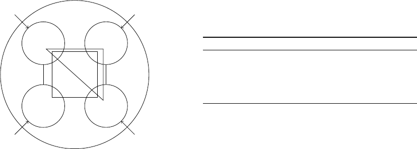
}. Figure 1 shows an example MOHN

where n = 4.

Figure 1: A four neuron MOHN with some of the weights

shown. w

is the triangle and w

is the square.

2.1 Using a MOHN

MOHNs can be applied to a number of different

computational intelligence tasks such as building a

content addressable memory, performing regression,

clustering, classiﬁcation, probability distribution es-

timation and as ﬁtness function models for use in

heuristic optimisation. These different tasks involve

different methods of use and require different ap-

proaches to estimating the values on the weights.

3 THE WEIGHT ESTIMATION

RULES

This section presents the different methods for es-

timating the weights needed to allow a MOHN to

perform a particular task. Although, in theory the

weights can be designed by hand, all of the methods

described here are based on learning from data. In

what follows, a single training example consists of a

vector of input variables and a real valued output de-

noted (x, y). The training data as a whole is denoted

3.1 Hebbian Learning

The simplest of the MOHN learning rules is an exten-

sion to the Hebbian rule employed by a Hopﬁeld net-

work to allow it to work with higher order weights. In

this case, the training data consists only of input pat-

terns, x and no function output is speciﬁed. Learning

involves setting u

= x

for each neuron and the weight

update is then:

= w

∏

u∈Q

u (2)

The Hebbian learning rule allows the MOHN to

be used as a content addressable memory (CAM). The

CAM learning algorithm is given in algorithm 1.

Algorithm 1: Loading Pattern x into a MOHN CAM.

= x

∀i  Set the neuron outputs to equal the

pattern to be learned

= w

∏

u∈Q

u ∀w

∈ W  Update the weights

according to equation 2

For a network that is fully connected at order two,

algorithm 1 is the same as loading patterns into a stan-

dard Hopﬁeld network. When the MOHN contains

higher order weights, the capacity of the network is

increased. Patterns are recalled as they are in a Hop-

ﬁeld network, by setting the neuron values to a noisy

or degraded pattern and allowing the network to set-

tle using a neuron update rule that ﬁrst calculates an

activation value for each neuron, a

using equation 3

and then applies a threshold using equation 4.

∑

j:u

∈Q

∏

k∈Q

(3)

NCTA 2015 - 7th International Conference on Neural Computation Theory and Applications

where j : u

∈ Q

makes j enumerate the index of each

weight that connects to u

and k ∈ Q

\ i indicates the

index of every member of Q

, except neuron i itself. A

neuron’s output is then calculated using the threshold

function in equation 4.



1, if a

> 0

−1, otherwise

(4)

An attractor state is a pattern across u from which

the application of equation 3 results in no change to

any of the neuron outputs. A trained MOHN settles to

an attractor point by repeated application of the acti-

vation rules 3 and 4, choosing neurons in random or-

der. Algorithm 2 describes the algorithm for settling

from a pattern to an attractor:

Algorithm 2: Settling a trained MOHN to an attractor point.

repeat

ch ← FALSE  Keep track of whether or not a

change has been made

visited ← {}  Keep track of which neurons

have been visited

repeat

i ← rand(i : i /∈ visited)  Pick a random

unset neuron

temp ← u

 Make a note of its value for

later comparison

Update(u

)  Update the neuron’s output

using equations 3 and 4

if u

6= temp then

ch ← T RUE

end if  If a change was made to the

neuron’s output, note the fact

visited ← {visited ∪ i}  Add the neuron’s

index to the visited set

until kvisitedk = n  Loop until all neurons

have been updated

until ch = FALSE  Loop if any neuron value has

changed

The dynamics of algorithm 2 have an underlying

Lyapunov function, just as they do in a standard HNN

and will always settle to a local minimum of the asso-

ciated energy function. (Venkatesh and Baldi, 1991)

report a capacity for binary valued order k networks

of the order of n

/ln n, a ﬁgure that is also reported

by (Kubota, 2007). In fact, as described below, such

networks are capable of representing any arbitrary

Lyaponov function and therefore a network with the

right structure will be able to represent any possible

number of turning points.

3.2 Weighted Hebbian Learning

Let f (x) be a multi-modal function where each lo-

cal maximum represents a pattern of interest. These

patterns might be local optima in an optimisation

task, archetypes in a clustering task or examples of

a satisfaction of multiple constraints, for example. A

MOHN can be trained as a CAM in which the attrac-

tors are the local maxima of the function. The learn-

ing rule is a weighted version of the Hebbian rule:

∑

x∈D

|D|

f (x)

∏

u∈Q

u (5)

Previous work (Swingler and Smith, 2014b) has

shown that the weighted Hebbian rule is capable of

learning the local maxima of a function from sam-

ples of x, f (x) and that the capacity of the resulting

networks for storing such attractors was equal to the

capacity of a CAM trained using equation 2. The dif-

ference between equations 2 and 5 is that the target

patterns are known in the ﬁrst case, but unknown in

the second, where they are local maxima of y in a

function that is learned from a sample of (x, y) pairs.

Note also that experiments have shown that the train-

ing data need not contain a single example of any of

the attractor patterns for the method to work.

3.2.1 Parity Count Learning

When the inputs (both single variables and products

of variable subsets) are uncorrelated (i.e. orthogonal)

and each input has an even distribution of values, the

weighted Hebbian rule produces the correct weight

values in a single pass of the data. When the distribu-

tion of values across each variable is uneven, a better

estimate of weight values may be made by taking into

account how often the input product on each weight

is positive or negative during learning. Each weight is

set to equal the difference between the average of the

output y when the weight’s input is positive and when

it is negative.

Let D

be the set of sub-patterns learned by w

that contain values whose product is positive and D

−

be the set of sub-patterns learned by w

that contain

values whose product is negative. Now let hy

i be the

average value of y associated with the members of D

and hy

−

i be the average value of y associated with the

members of D

−

i =

∑

x∈D

f (x) (6)

Similarly, hy

−

i is calculated as a sum over

x ∈ D

−

. The weight calculation is simply

A Comparison of Learning Rules for Mixed Order Hyper Networks



i − hy

−



(7)

The averages may be maintained online so that the

weight values are always correct at any time during

learning (rather than summing and dividing at the end

of a deﬁned training set). W

is set in a similar way.

The Weighted Hebbian calculation, w

= hyi means

that w

is just the average of the output, y across the

training sample. This can be improved by taking into

account the distribution of patterns across each input.

= hyi −

∑

j:w

∈W



∏

x∈w



(8)

where x ∈ w

indicates the neurons connected to

weight w

and



∏

x∈w



is the average value across

all input patterns of the product of the values of x con-

nected to w

3.3 Regression Rules

The weighted Hebbian update rule is capable of cap-

turing the turning points in a function, but cannot ac-

curately reproduce the output of the function itself

across all of the input space. Such networks have an

energy function

and this can be used as a regression

function for estimating ˆy = f (x) in the form

ˆy =

∑

∏

u∈Q

u (9)

The weight values for the regression may be cal-

culated either in a single off line calculation or using

an on line weight update rule.

3.3.1 Off Line Regression

To use ordinary least squares (OLS) (Hastie et al.,

2009) to estimate the weights ofﬂine, a matrix X is

constructed where each row represents a training ex-

ample and each column represents a weight. The ﬁrst

column represents W

and always contains a 1. The

remaining columns contain the product of the val-

ues of the inputs connected by the column’s weight,

∏

x∈Q

x. A vector Y takes the output values associ-

ated with each of the input rows and the parameters

are calculated using singular value decomposition:

β = (X

−1

y (10)

where X

is the transpose of X, X

−1

is the inverse

of X and β becomes a vector from which the weights

of the MOHN may be directly read so that w

= β

The regression equation 9 is actually the negative of

the energy function, which is minimised by applying the

settling algorithm 2.

and the remaining weights take values from β in the

same sequence as they were inserted into the matrix

3.3.2 LASSO Learning Rule

The LASSO algorithm (Tibshirani, 1996) may also be

used to learn the values on the weights of the MOHN.

Each input vector is set up in the same way as de-

scribed for OLS, by calculating the product of the

input values connected to each weight and the coef-

ﬁcients generated by LASSO are read back into the

weights of the MOHN in the same order. LASSO per-

forms regression with an additional constraint on the

norm of the weight vector. The learning algorithm

minimises the sum:

∑

x∈D

( f (x) −

f (x)) + λ

∑

w∈W

|w| (11)

where λ controls the degree of regularisation. When

λ = 0, the LASSO solution becomes the OLS solu-

tion. With λ > 0 the regularisation causes the sum of

the absolute weight values to shrink such that weights

with the least contribution to error reduction take a

value of zero. This not only allows LASSO to re-

ject input variables that contribute little, but also to re-

ject higher order weights that are not needed. LASSO

can be used as a simple method for choosing network

structure by over-connecting a network and then re-

moving all the zero valued weights after LASSO re-

gression has been performed.

3.3.3 On Line Learning

The weights of a MOHN can also be estimated on

line (where the data is streamed one pattern at a time,

rather than being available in a matrix as in equation

10) using a linear version of the delta learning rule,

the Linear Delta Rule (LDR):

= w

+ α( f (x) −

f (x))

∏

u∈Q

u (12)

where α < 1 is the learning rate. Experimental re-

sults have suggested that one divided by the number

of weights in the network is a good value for α, i.e

α =

|W |

. This allows the correction made in response

to each prediction error to be spread across all of the

weights.

The online learning algorithm is very similar to

the perceptron (or MLP) learning algorithm. The iter-

ative nature of the algorithm allows for early stopping

to be used to control for overﬁtting with reference to

an independent test set. Algorithm 3 describes the

learning process.

NCTA 2015 - 7th International Conference on Neural Computation Theory and Applications

Algorithm 3: On Line MOHN Learning with the Linear

Delta Rule.

Let D

be a subset of the available data to be used

for training the network

Let D

be a subset of the available data to be used

for testing the network

for all (x, f (x)) ∈ D

Initialise the weights in the network using the

parity rule of equation 7

end for

repeat

for all x ∈ D

Update the weights in the network using the

delta learning rule of equation 12

Let e be the root mean squared error that

results from evaluating every member of D

with

the model

end for

until e is sufﬁciently low or starts to increase con-

sistently

Note that the weights are initialised with the par-

ity count learning rule, not to random values as with

an MLP. This is because there are no local minima in

the error function and so no need for random starting

points. In cases where the entire input,output space

of the function may be noiselessly sampled, the ini-

tialisation step will produce the correct weights imea-

diately, without the need for additional error descent

learning. The learning algorithm will work without

the initialisation (the weights can be set to zero) but

then requires more iterations of the learning cycle.

4 ANALYSIS OF LEARNING

RULES

This section begins with a summary of the abilities

and limitations of the different learning rules pre-

sented in this paper. It then goes on to analyse the

rules and the resulting networks. Table 1 summarises

some of the differences between the methods. Due

to the structure of the MOHN, all of the learning rules

are capable of reproducing the maximal turning points

of the learned function, but the Hebbian based rules

do not minimise the error elsewhere in the function

space. The Hebbian rules learn in a single presenta-

tion of the data, so can operate in an on line mode

without the need to iterate through the data set more

than once. The others require either on line iterations

or the entire data set to be present off line.

The weighted Hebbian rule is accurate only when

a full sample of the input/output space is available,

Table 1: Comparing four different MOHN learning rules in

terms of the learning mode, any regularisation that is pos-

sible, whether or not the training error is minimised, and

whether the training data is presented as input,output pairs

(IO) or as patterns to store in a content addressable memory

(CAM).

Method Mode Reg. Min. Err. Data

Hebbian One shot None No CAM

Weighted Hebb One shot None No IO

LDR On line Early Stop Yes IO

OLS Off line None Yes IO

LASSO Off line L

-norm Yes IO

so is of limited practical use as the parity counting

method gives more accurate estimates operating on

weights independently with a single pass through the

data. The parity counting method provides good start-

ing weights for the linear delta rule.

The following sections investigate different net-

work structures in more detail.

4.1 Second Order Networks

When a MOHN has only second order connections,

it is equivalent to a Hopﬁeld Neural Network (HNN)

(Hopﬁeld, 1982) and the Hebbian learning rule of

equation 2 is the standard learning rule for a HNN.

It is well known that HNNs are able to learn patterns

as content addressable memories, but that they suffer

from the presence of spurious attractors too. These

spurious attractors may be removed (or their presence

avoided) by deﬁning an energy function for the net-

work in which the patterns to be stored as memories

are local maxima. This may be done using a Ham-

ming distance based function and (Swingler, 2012),

(Swingler and Smith, 2014b) have shown that using

the weighted Hebbian update rule of equation 5 and

such a function on a second order MOHN (or equiv-

alently, a HNN) is sufﬁcient to produce a content ad-

dressable memory in which the turning points of the

function are the memories to be stored. The capac-

ity of a HNN for storing patterns is the same if the

patterns are loaded directly with the Hebbian learn-

ing rule as it is when the patterns are learned from a

Hamming distance based function.

To build the Hamming distance based function,

denote the set of patterns to be stored as T:

T = {t

,... ,t

} (13)

and deﬁne a set of sub-functions, f (x|t

) as a

weighted Hamming distance between x and each tar-

get pattern t

in T as

f (x|t

) =

∑

(14)

A Comparison of Learning Rules for Mixed Order Hyper Networks

where t

is element i of target j and δ

is the Kro-

necker delta function between pattern element i in t

and its equivalent in x. The function output given an

input pattern, f (x) is the maximal output across all

the sub-functions given an input of f (x).

f (x|t) = max

j=1...s

( f (x|t

)) (15)

By generating random input patterns, evaluating

each using equation 15 and then using the LDR of

equation 12 to learn each input,output pair sampled,

a network with attractors at each member of T is

learned. The network has the additional quality that

as the number of samples learned increases, the num-

ber of spurious attractors in the network decreases.

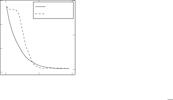
To test this claim, experiments were run in which

a 100 neuron MOHN was trained on a function that

contained four true attractor states. Figure 2 shows

the average results of running 100 trials in which the

number of spurious attractors and the error of the net-

work were measured for each iteration of the training

data, which was a random sample of size 20,000 from

the Hamming distance based function 15. In each

case, the number of spurious attractors was reduced

to zero as the training error approached zero.

100

0.1

0.2

0.3

Training Epoch

Training Error

500

1,000

Spurious Attractors

Error

Attractors

Figure 2: As the number of learning iterations increases,

the training error decreases as does the number of spurious

attractors in the model.

Researchers have shown how the weights of a

HNN can be designed to represent the travelling sales-

man problem (Hopﬁeld and Tank, 1985), (Wilson

and Pawley, 1988) and other problems such as graph

colouring (Caparr

os et al., 2002). These approaches

are limited by the fact that the weights must be cho-

sen by hand to reﬂect the constraints of the problem

to be solved. By training a HNN (or a MOHN) by

sampling from a ﬁtness function, it is now possible to

build a network to represent any problem with a ﬁt-

ness function that can be evaluated, not just those that

are amenable to having their weights set by hand.

4.2 Full Networks

When the data are noise free, a network is fully con-

nected and the data sample is exhaustive (i.e. it covers

every possible input pattern once), the weighted Heb-

bian rule of equation 5 (with |D| = 2

) will produce

weights which reproduce the target function perfectly.

In such cases, the product

∏

u∈Q

u provides a basis

function for f : {−1, 1}

→ R. This basis function

is very similar to the well know Walsh basis (Walsh,

1923), (Beauchamp, 1984).

A Walsh representation of a function f (x) is de-

ﬁned by a vector of parameters, the Walsh coefﬁ-

cients, ω = ω

...ω

−1

. Each ω

is associated with

the Walsh function ψ

. The Walsh representation of

f (x) is constructed as a sum over all ω

. In the sum,

each ω

is either added to or subtracted from the total,

depending on the value of the Walsh function ψ

(x)

which gives the function for the Walsh sum:

f (x) =

n−1

∑

j=0

(x) (16)

A Walsh function, ψ

(x) returns +1 or -1 depend-

ing on the parity of the number of 1 bits in shared

positions across x and j where j is the binary repre-

sentation of the integer j. Using logical notation, a

Walsh function is derived from the result of an XOR

(parity count) of an AND (agreement of bits with a

value of 1):

(x) = ⊕

i=1

∧ j

) (17)

where ⊕ is a parity operator, which returns 1 if the

argument list contains an even number of 1s and -1

otherwise. The Walsh transform of an n-bit function,

f (x), produces 2

Walsh coefﬁcients, ω

, indexed by

the 2

combinations across f (x). Each Walsh coefﬁ-

cient, ω

is calculated by

−1

∑

x=0

f (x)ψ

(x) (18)

The weight values in a fully trained MOHN are

equal in magnitude to the Walsh coefﬁcients of the

same index, but that they differ in sign when the

weight order is an odd number. That is,

= p(ω

∀w

∈ W (19)

where p(ω

) is the parity of the order of ω

such that:

p(ω

) =

(

1 if the order of i is even

−1 otherwise

(20)

This is because the Walsh function returns a value

based on a parity count of the number of variables set

NCTA 2015 - 7th International Conference on Neural Computation Theory and Applications

to one across the input variables that are connected to

a given coefﬁcient, as shown in equation 17. The par-

ity function returns 1 if the number of variables with

a value of one is even and -1 otherwise. The MOHN

uses the product of those same values, which evalu-

ates to -1 whenever there is an odd number of inputs

set to -1. The MOHN indices match the Walsh coefﬁ-

cient indices because they both use the same method

of deriving the index number from the binary repre-

sentation of the connections described in section 2.

As a fully connected MOHN provides a basis for

all possible functions in f : {−1,1}

→ R, then it fol-

lows that any function with coefﬁcient values of zero

may be perfectly represented by a less than fully con-

nected MOHN so providing the correct structure can

be found, a MOHN may represent any arbitrary func-

tion.

4.3 Discovering Network Structure

The structure of a MOHN is deﬁned by W , which

is a subset of all possible 2

weights. As noted

above, a fully connected second order network im-

plements a HNN and a fully connected network at all

orders forms a basis of all functions f : {−1, 1}

→ R.

Any other pattern of connectivity is also possible, for

example a ﬁrst order only network is equivalent to

a perceptron, or a multiple linear regression model.

Adding higher order weights increases the power of

the model to represent more complex functions.

Discovering the correct structure for the network

is both challenging and instructive, compared to the

same task when using an MLP, which is quite straight

forward, but done in the dark. The question of dis-

covering structure in functions from samples of data

is of particular importance in the ﬁeld of metaheuris-

tic optimisation, where it is called linkage learning

(see (Pelikan et al., 2000), (Heckendorn and Wright,

2004)).

The correct structure for a function may be dis-

covered from the training data using an iterative ap-

proach of adding and removing weights as training

progresses. The basics of the structure discovery al-

gorithm are to train a partial network, test the signif-

icance of the weights it contains, remove those that

are not signiﬁcant, then add new weights according

to some criteria. The weight picking criteria chosen

for this work are based on maintaining a probability

distribution over the possible weights, which is up-

dated on each round of learning so that connection

orders and neurons that have proved useful in previ-

ous rounds have a higher probability of being picked

in subsequent rounds. The process is described in al-

gorithm 4.

Algorithm 4: Probability distribution based structure dis-

covery algorithm.

Start with an empty network with weight set W =

Initialise a distribution over possible weights, P(w)

repeat

Sample new weights from the distribution P(w)

Calculate the values for all weights

Remove any insigniﬁcant weights from the net-

work

Update the weights distribution, P(w)

Calculate the test error

until The test error is sufﬁciently low or doesn’t

change

The probability distribution over W is based on

the order of a weight and the neurons it connects. The

sampling process involves ﬁrst picking an order, k for

the weight to be added from a distribution, Pk() over

all possible orders (1... n) and then picking k neu-

rons to connect from a distribution, Pn() over the n

available neurons. The choice made for the algorithm

described here is to impose an exponential distribu-

tion on the choice of weight order, centred at order

c where initially c = 1 and c is incremented as lower

order weights are either used or discarded.

Pk(k) = λe

−λ|c−k|

(21)

where λ controls the width of the distribution. In the

early iterations of the algorithm where c = 1, there

is a high probability of picking ﬁrst order weights

and an exponentially decreasing probability of pick-

ing weights of higher order. In subsequent itera-

tions, Pk(k) is updated in two ways. Firstly, c is

incremented to allow the algorithm to pick weights

with higher orders and secondly the values of existing

weights are used to shape the distribution to guide the

algorithm towards orders that have yielded high value

weights already.

The weight order probability distribution, Pk(k) is

updated by counting the proportion of weights in the

current network that are of each order. Let this vector

of proportions be p = p

... p

where p

is the number

of weights at order i divided by the total number of

weights in the network. These proportions are then

used to update Pk() as follows along with an updated

version of the exponential distribution:

Pk(i) ← (1 − (α + β))Pk(i) + αp

+βλe

−λ|c−k|

(22)

where α and β are update rates such that 0 ≤ α ≤ 1,

0 ≤ β ≤ 1 and 0 < α + β ≤ 1.

The neuron distribution update rule sets the prob-

ability of a neuron being picked to be proportionate

A Comparison of Learning Rules for Mixed Order Hyper Networks

to the sum of the absolute values of the weights con-

nected to it. The contribution of neuron i is C(i)

C(i) =

∑

∈w

|w| (23)

and the probability of picking neuron i is

Pn(i) =

C(i)

∑

n−1

j=0

C( j)

(24)

As each new set of weights is added, another

phase of learning cycles is required to update the new

network. The existing weight values will be close

to their correct value, but need to change slightly to

accommodate the newly added weights. The new

weights also need to be learned. This is requires an on

line learning approach as the existing weights need to

be moved from their current values, rather than cal-

culated from scratch, making the delta rule the ideal

choice. Weights may be identiﬁed for removal by per-

forming a t-test on their values, looking for signiﬁcant

difference from zero in order to keep a weight. Al-

ternatively, each new structure may be learned from

scratch using LASSO, which has the advantage of au-

tomatically identifying the weights to remove as those

with a coefﬁcient of zero.

This approach to growing a neural network differs

from the many previously reported methods in that it

only adds weights, not neurons. Generally, grow-and-

learn neural network algorithms proceed by adding

neurons to the existing hidden layer or by introduc-

ing new layers. For example the Netlines algorithm

(Torres-Moreno and Gordon, 1998) adds binary hid-

den units one at a time in an incremental approach to

learning classiﬁer functions. The Upstart algorithm

(Frean, 1990), on the other hand, produces deeper tree

structured networks by adding pairs of hidden units

between the input layer and the current ﬁrst hidden

layer. As a MOHN contains no hidden units, it is only

weights, not neurons that are added at each iteration

of the growth algorithm.

The MOHN may also be compared to other sta-

tistical models. By introducing a link function, a

MOHN becomes a generalised linear model (GLM)

(Dobson and Barnett, 2011). A link function is usu-

ally a non-linear function that is applied to the output

of a linear regression to allow a wider range of proba-

bility distributions to be modelled. The general form

g(x) = ˆy (25)

where ˆy is the energy function of the network from

equation 9 and g(x) is the link function. If the in-

verse of g (x) is known, then the learning rules may

all be used with the simple replacement of f (x)

with g

−1

( f (x)). For example, setting g(x) = e

and

−1

(x) = ln(x) constructs a Boltzmann distribution if

the target values, f (x) are proportional to the prob-

ability of pattern x. This is the approach taken in

(Shakya et al., 2012) who use a Markov Random

Field to model the distribution of solutions to opti-

misation problems by training a mixed order network

with an exponential link function using OLS.

5 EXPERIMENTAL RESULTS

In this section, the learning rules described in this pa-

per are compared with each other and with a standard

multi layer perceptron (MLP) for the speed at which

they learn. The Hamming distance based function of

equation 15 was used for these tests as it is possible to

generate arbitrary functions containing a chosen num-

ber of turning points at random locations. This allows

the different methods to be tested across thousands of

different functions of varying degrees of complexity.

5.1 Speed Against Complexity

One way to vary the complexity of a function is to

vary the number of turning points it contains. This

section describes a set of experiments designed to

measure the speed of learning of each of the MOHN

learning rules and an MLP as the complexity of the

function to be learned varies. Each single experiment

involved training a MOHN and an MLP on a data set

generated from a function with a random number of

turning points. The same data was used to train three

different MOHNs, one with each learning rule from

OLS, LASSO and LDR. The function had 15 inputs

and the MOHNs were fully connected up to order

three, giving them 576 weights. The MLP has only

10 hidden units, giving it only 176 weights.

A sample of 580 random points was used for train-

ing each network. For the iterative learning methods

(all except OLS) a target error of 0.01 was used as a

stopping criteria, hence the measure of interest was

time taken to reach a training error of 0.01. This pro-

cess was repeated 1000 times, each with a new func-

tion with a number of turning points between 1 and

30.

Figure 3 shows the results. All methods except

the MLP learned the function in a constant time, re-

gardless of the degree of complexity. The MLP was

able to learn the single turning point function (i.e. lin-

ear function) in less time than it was able to learn the

more complex functions. The function with two turn-

ing points was also faster than those with more. After

NCTA 2015 - 7th International Conference on Neural Computation Theory and Applications

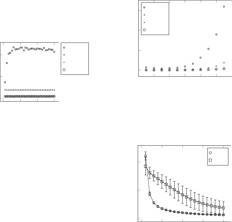
two turning points, the learning time for the MLP be-

came constant. Regardless of the complexity of the

function, the MLP always took considerably longer,

followed by OLS. The LDR and LASSO algorithms

took similar amounts of time and were the fastest.

0 10 20 30

1,000

2,000

Turning Points

Training Time

Learning Time by Complexity

MLP

OLS

LASSO

LDR

Figure 3: Average learning time in milliseconds by function

complexity for different MOHN learning rules and an MLP.

The LASSO and LDR values are almost equal and can be

seen along the bottom of the graph.

5.2 Speed By Network Size

Another set of similar experiments related the training

speed of each method to the size of the network. The

number of inputs to a network was varied from 5 to

15 and 1000 trials were run. The mean squared error

of the result of performing OLS was used as the stop-

ping criteria for the MLP and the MOHN as it was

trained with LDR, ensuring that all models had the

same level of accuracy. Figure 4 shows the results.

OLS is known to have a time complexity of O(np

)

where n is the number of data points and p is the num-

ber of variables. LASSO and LDR were of the same

order, but the algorithms ran in less time. The MLP’s

training time grew exponentially with the number of

variables in these particular experiments. As before

the MOHN models all reached the target training er-

ror faster than the MLP.

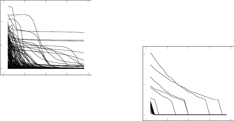
5.2.1 Error Descent Rate

The difference in training speed between the MOHN

and an MLP was investigated further by recording the

average error by training epoch for the ﬁrst twenty

passes through the training data. Figure 5 shows the

average error on each pass of the training data from

1000 repeated trials on functions of varying complex-

ity. The error bars show 1 standard deviation from

the mean. Note that the MOHN error drops faster and

that there is far less variation across trials (the error

8 10 12 14

1,000

2,000

3,000

Input Variables

Training Time

Learning Time by Network Size

MLP

OLS

LASSO

LDR

Figure 4: Average learning time in milliseconds by number

of inputs for different MOHN learning rules and an MLP.

bars for the MOHN are sufﬁciently short that they sit

inside the marks).

0.2

0.4

Training Epochs

Training Error

Training Error by Epoch

LDR

MLP

Figure 5: The mean and standard deviation of training error

as it descends over twenty training epochs, comparing an

MLP with the Linear Delta Rule training a MOHN.

The improved learning speed of the MOHN and

the slower, more varied speed of the MLP may be

explained by the fact that the MLP combines ﬁtting

parameter values with feature selection. Recently,

(Swingler, 2014) provided an insight into the phases

of MLP training, showing that early training cycles

are taken up with ﬁxing the role of the hidden units

and later cycles then ﬁt the parameters within the con-

straints of the features encoded by those hidden units.

The MOHN does not have hidden units and so only

needs to ﬁt parameter values to its ﬁxed structure. Of

course, that structure needs to be discovered, but the

task of structure discovery and parameter ﬁtting are

separated, unlike the case for the MLP.

Another consequence of the MLP’s dual learning

A Comparison of Learning Rules for Mixed Order Hyper Networks

500

1,000

1,500

2,000

0.00

0.05

0.10

Training Epoch

Training Error

Training Error Descent for MLP

Figure 6: Traces of training error over 200 different at-

tempts at training an MLP on a concatenated XOR function.

Note the variation in convergence time and the presence of

a number of failed attempts after 2000 epochs.

task of ﬁtting both function structure and regression ﬁt

is that the error function contains local minima. These

occur when the hidden units encode a suboptimal set

of features and the network ﬁts weight values to them.

This is commonly solved by re-starting the training

process from a different random set of initial weight

values. The MOHN error function does not contain

local minima, so the weights do not need to be ran-

domised before learning, as shown in algorithm 3. To

illustrate this point, a ﬁnal set of experiments com-

pared an MLP trained with error back propagation to

a MOHN trained with the LDR on a function designed

to contain local minima in its cost function. The func-

tion to be learned was a concatenation of XOR pairs

such that each x

where i is even is paired with x

i+1

to form an XOR function. The function output is the

normalised sum of the XOR of the pairs, so 101010

would produce an output of one and 110011 would

produce zero. Figure 6 shows the traces of 200 MLPs

started with random weights, each trained for 2000

cycles through the training data. The variation in er-

ror descent is clear, with some networks converging

quickly, some taking many training epochs to con-

verge, and some still stuck in local minima after 2000

epochs.

For functions of small numbers of inputs, it was

possible to exhaustively sample the function space

and so use the weighted Hebb rule to allow the

MOHN to learn the function fully in a single pass of

the data. For networks where the number of inputs is

too large for an exhaustive sample, a random sample

was taken. Figure 7 shows the trace of the training

error during 200 attempts at learning the same XOR

based function as that in ﬁgure 6 using a MOHN with

the LDR. The variation is not due to random starting

points—all networks start with weights at zero—but

is due to the fact that the training data is a small ran-

dom subset of the full input space. Note that there are

no traces that indicate a local minimum; all go to zero

error.

100

150

200

0.000

0.002

0.004

Training Epoch

Training Error

Training Error Descent for MOHN

Figure 7: Traces of training error over 200 different at-

tempts at training a MOHN on a concatenated XOR func-

tion. Compare both the scale of the error and the number of

training epochs involved with the same plot for the MLP in

ﬁgure 6.

6 SUMMARY AND FUTURE

DIRECTIONS

Mixed Order Hyper Networks are universal function

approximators over f : {−1,1}

→ R. They may be

trained from a sample of data to act as either a re-

gression function that attempts to ﬁt the function that

underlies the data across the entire function space or

just to capture the function’s turning points as energy

minima. Learning may be off line, in which case all

of the data needs to be available at one time, or on

line in situations where data is streamed or the net-

work structure is changing and existing weights need

to be updated. This paper presented ﬁve learning rules

designed to cover both on line and off line learning,

and both regression and content addressable memory

learning. Other learning methods might also be con-

sidered such as ridge regression or LARS, but that is

left for future work.

This paper has only presented networks for func-

tion learning, but they may also be used as classiﬁers.

As a MOHN has only one output, binary classiﬁca-

tions are straight forward. Further work is required

to discover the best way to learn multi-class models.

Learning a classiﬁer will also introduce the possibility

NCTA 2015 - 7th International Conference on Neural Computation Theory and Applications

of using alternative learning algorithms such as Min-

imerror (Torres-Moreno et al., 2002), which is a per-

ceptron learning rule with a cost function designed to

reduce the number of classiﬁcation errors rather than

mean squared error. The MOHN and its learning rules

would also be usefully compared to deep networks as

they present a start contrast in approach.

The issue of MOHN structure discovery was also

raised, but the detail is left for future work. The exper-

iments presented in this paper worked on the assump-

tion that the networks in question contained weights

of sufﬁcient order to capture the functions on which

they were trained. This becomes increasingly difﬁcult

as the number of inputs grows. Problems with large

numbers of inputs require a structure discovery phase

to be carried out as part of the training process.

With a given network structure, training a MOHN

is faster and has less error variance across trials than

training with an MLP. Additionally, the training al-

gorithm has no local minima when training a ﬁxed

structure MOHN, making training more reliable than

that of an MLP. Of course, any algorithm used to dis-

cover the correct structure for the MOHN may well

have local optima, but that (again) is a matter for fu-

ture work.

REFERENCES

Beauchamp, K. (1984). Applications of Walsh and Related

Functions. Academic Press, London.

Caparr

os, G. J., Ruiz, M. A. A., and Hern

andez, F. S.

(2002). Hopﬁeld neural networks for optimization:

study of the different dynamics. Neurocomputing,

43(1-4):219–237.

Dobson, A. J. and Barnett, A. (2011). An introduction to

generalized linear models. CRC press.

Frean, M. (1990). The upstart algorithm: A method for con-

structing and training feedforward neural networks.

Neural computation, 2(2):198–209.

Hastie, T., Tibshirani, R., Friedman, J., Hastie, T., Fried-

man, J., and Tibshirani, R. (2009). The elements of

statistical learning, volume 2. Springer.

Heckendorn, R. B. and Wright, A. H. (2004). Efﬁcient link-

age discovery by limited probing. Evolutionary com-

putation, 12(4):517–545.

Hopﬁeld, J. J. (1982). Neural networks and physical sys-

tems with emergent collective computational abili-

ties. Proceedings of the National Academy of Sciences

USA, 79(8):2554–2558.

Hopﬁeld, J. J. and Tank, D. W. (1985). Neural computa-

tion of decisions in optimization problems. Biological

Cybernetics, 52:141–152.

Kubota, T. (2007). A higher order associative memory with

Mcculloch-Pitts neurons and plastic synapses. In Neu-

ral Networks, 2007. IJCNN 2007. International Joint

Conference on, pages 1982 –1989.

Pelikan, M., Goldberg, D. E., and Cant

u-paz, E. E.

(2000). Linkage problem, distribution estimation,

and bayesian networks. Evolutionary Computation,

8(3):311–340.

Shakya, S., McCall, J., Brownlee, A., and Owusu, G.

(2012). Deum - distribution estimation using markov

networks. In Shakya, S. and Santana, R., editors,

Markov Networks in Evolutionary Computation, vol-

ume 14 of Adaptation, Learning, and Optimization,

pages 55–71. Springer Berlin Heidelberg.

Swingler, K. (2012). On the capacity of Hopﬁeld neural

networks as EDAs for solving combinatorial optimi-

sation problems. In Proc. IJCCI (ECTA), pages 152–

157. SciTePress.

Swingler, K. (2014). A walsh analysis of multilayer percep-

tron function. In Proc. IJCCI (NCTA), pages –.

Swingler, K. and Smith, L. (2014a). Training and making

calculations with mixed order hyper-networks. Neu-

rocomputing, (141):65–75.

Swingler, K. and Smith, L. S. (2014b). An analysis of

the local optima storage capacity of hopﬁeld network

based ﬁtness function models. Transactions on Com-

putational Collective Intelligence XVII, LNCS 8790,

pages 248–271.

Tibshirani, R. (1996). Regression shrinkage and selection

via the lasso. Journal of the Royal Statistical Society.

Series B (Methodological), pages 267–288.

Torres-Moreno, J.-M., Aguilar, J., and Gordon, M.

(2002). Finding the number minimum of errors in n-

dimensional parity problem with a linear perceptron.

Neural Processing Letters, 1:201–210.

Torres-Moreno, J.-M. and Gordon, M. B. (1998). Efﬁcient

adaptive learning for classiﬁcation tasks with binary

units. Neural Computation, 10(4):1007–1030.

Venkatesh, S. S. and Baldi, P. (1991). Programmed inter-

actions in higher-order neural networks: Maximal ca-

pacity. Journal of Complexity, 7(3):316–337.

Walsh, J. (1923). A closed set of normal orthogonal func-

tions. Amer. J. Math, 45:5–24.

Wilson, G. V. and Pawley, G. S. (1988). On the stability of

the travelling salesman problem algorithm of hopﬁeld

and tank. Biol. Cybern., 58(1):63–70.

A Comparison of Learning Rules for Mixed Order Hyper Networks