Aerodynamical Resistance in Cycling

CFD Simulations and Comparison with Experiments

Luca Oggiano, Live Spurkland, Lars Sætran and Lars Morten Bardal

Norwegian University Of Science and Technology, Deparment of Energy and Process Engineering,

K. Hejes Vei 2b, 7042 Trondheim, Norway

Keywords: Aerodynamics, CFD, Wind Tunnel Testing, Cycling.

Abstract: The present work shows a comparison between computational fluid dynamics (CFD) simulations obtained

using the Unsteady Reynolds Averaged Navier-Stokes solver STARCCM+ from CD-Adapco and

experiments carried out in the subsonic wind tunnel at NTNU. The models tested in the wind tunnel (a

mannequin and real cyclist in static position) were 3D scanned using a 3D scanner, consisting 48 single-lens

reflex cameras surrounding the object in three heights (low/ground-midi-above). A hybrid meshing

technique was used in order to discretize the surface and the volume. Polyhedral cells were used on the

model surface and in the near volume while a structured grid was used in the rest of the domain. An

unsdeady RANS approach was used and the turbulence was modelled using the Menter implementation of

the k-ω model. No wall functions were used and the boundary layer was fully resolved. The first part of the

paper focuses on the mannequin while in the second part the comparison between the experimental results

and simulation on the real cyclist are presented. An overall good agreement between the simulations and the

experiments was found proving that CFD could be a complementary tool to wind tunnel testing.

1 INTRODUCTION

The aerodynamic drag is the main opposing force

that cyclists need to overcome and it counts up 90%

((De Groot et al., 1995, Di Prampero, 2000; Oggiano

et al., 2008)) of the total resisting forces experienced

by a cyclist at racing speeds. The cyclist itself counts

up to 70% of the total drag while the remaining 30%

is due to the bicycle (Blocken et al., 2013;

Underwood, 2012; Underwood and Jermy, 2011;

Oggiano et al., 2008) and this leads to the fact that

even small reductions could give large

improvements in terms of performances.

The aerodynamic drag generated by the cyclist is

directly linked to a number of parameters.

Expressing the drag as

(1)

It can be immediately noticed that, for a given

location where the air density  [kg/m

] is assumed

to be constant, the drag is proportional to the square

of the wind speed U [m/s], to the frontal area A [m

]

and to the non-dimensional drag coefficient C

[-].

Being the frontal area measurements often not

reliable (Debraux et al., 2012), a combined

parameter called arag area C

A is used to quantify

the effectiveness of a cycling posture.

In order optimize their posture with the main goal

to reduce the drag area (and thus the drag),

experimental tests became common amongst elite

cyclists. Different methods of assessment of

aerodynamic drag (wind tunnel tests, linear

regression analysis models, traction resistance

measurement methods and deceleration methods) are

currently used and each of them has pros and cons

(Debraux et al., 2012).

Beside experimental methods, Computational

Fludi Dynamics (CFD) simulations became a viable

option due the increase in computational power

available and to the possibility to parallelize the

simulations splitting large meshes into smaller

domains. Encouraging results from CFD simulations

applied to cycling can be found in (Hanna, 2002;

Defraeye et al., 2010a; Defraeye et al., 2010b;

Defraeye et al., 2011; Lukes et al., 2002; Blocken et

al., 2013)

and while applications in other sports have

been carried out by a number of other authors

(Lecrivain et al., 2008; Minetti et al., 2009; Zaïdi et

al., 2010)

CFD simulations present some pros and some

cons if compared with wind tunnel tests. While wind

 0.5c



Oggiano, L., Bardal, L., Sætran, L. and Spurkland, L..

Aerodynamical Resistance in Cycling - CFD Simulations and Comparison with Experiments.

In Proceedings of the 3rd International Congress on Sport Sciences Research and Technology Support (icSPORTS 2015), pages 183-189

ISBN: 978-989-758-159-5

183

tunnel tests are able to provide only the total drag

force acting on the model, CFD can provide drag

information on individual body segments or bicycle

components, increasing the insight in drag reduction

mechanisms and allowing local modifications.

Furthermore, CFD simulations are able to provide

instantaneous field data while wind tunnel tests are

not. On the other hand, the main disadvantage of

CFD versus wind tunnel tests is that moving athletes

are extremely complex to simulate and thus

simulations are confined to static models. The other

main issue is that, in order to reduce the

computational cost of the simulations, turbulence

has to be modelled and cannot be fully resolved.

This simplification has two main drawbacks: the

separation lines on the model will be placed

considering the flow around the model fully

turbulent (not always true in reality) and, even with

the use of surface roughness and transition models,

drag reduction techniques (Oggiano and Sætran,

2012; Oggiano et al., 2009; Brownlie, 1992;

Brownlie et al., 1987; Brownlie et al., 2009) cannot

be simulated or directly implemented in the

simulation.

The present work aims to validate CFD

simulations towards experiments proving the

effectiveness of CFD as a complementary rather

than a substitute tool to wind tunnel tests.

2 EXPERIMENTAL SETUP

Testing of the mannequin models and cyclist were

conducted in the large wind tunnel at NTNU. The

wind tunnel is equipped with a 220KW fan engine,

has a maximum speed of 30m/s and the testing

section is 2,7x1,8x12,5 meters. A pitot tube and a

thermocouple type K was used to monitor the wind

speed and temperature respectively. The drag was

measured with a Schenck six component force

balance where only the axis of the drag direction

was used. The drag force was calculated from the

measured CdA values and normalized

2.1 Mannequin Model

The test on the mannequin model were conducted on

five velocities ranging from 9.53 to 18.2 m/s

(corresponding to 35 to 72,5 km/h).

The mannequin model used for the test was a

full-scale upper body including head and upper arms

belonging to a model of height 170 cm and weight

70 kg. Its position was adjusted to imitate that of a

cyclist in the drop bars. The forearms were removed

to reduce the amount of uncertainty and helmets

were not included in the test. The model was tested

with a number of jerseys with different surface

pattern and without jersey with different rough

patches applied to the shoulder. Its position was

adjusted to resemble the dropped position of a

cyclist.

2.2 Mannequin Model

The full scale test on a cyclist was carried out at a

single wind speed (13.09m/s). A regular road bike

was placed on a training roller so that the tires were

not touching the wind tunnel floor and the roller was

connected to the force plate. The front wheel was

stationary and supported by a custom-made wheel

stand. The cyclist was positioned in drop positon

with live pictures from a side camera projected in

front of the rider showing their position

superimposed with an outline of her initial position

to keep it as consequent as possible.

3 NUMERICAL SETUP

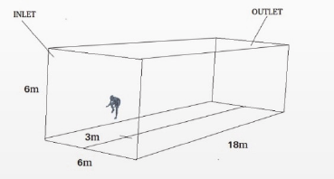
3.1 Computational Domain and

Geometry

Figure 1: Numerical wind tunnel.

The numerical simulations were set up for a

cyclist without bicycle setup and for a mannequin

without support setup. The bike modelling was

discarded in order to reduce the mesh size and thus

the computational cost of the simulation. However,

due to this approach, the interaction between the

bike and the cyclist was discarded and simplified.

No roughness was added to the model while it has

been previously shown that roughness could be a

key factor and dramatically affect the drag

(Brownlie, 1992; Brownlie et al., 1987; Brownlie et

al., 2009). The digital models for mannequin and

cyclist were obtained using a high-resolution 3D

laser scanning. The cyclist and mannequin digital

models were placed in a numerical wind tunnel. A

icSPORTS 2015 - International Congress on Sport Sciences Research and Technology Support

184

preliminary study on the domain size was carried out

in order to avoid backflow that could affect the

simulation. The domain shape and size is specified

in Figure 1.

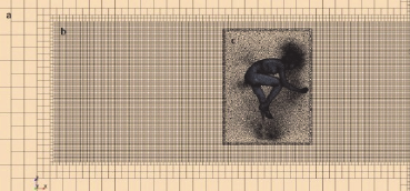
3.2 Mesh and Grid Sensitivity

Figure 2: Mesh refinement technique a) farfield area

(structured mesh). b) wake area (structured mesh). c) Near

model area (unstructured polyhedral mesh).

A hybrid meshing approach was used to mesh

the cyclist and the wind tunnel. A polyhedral

meshing approach was used to discretize the models

surface while a structured hexaedra approach was

used for the rest of the domain. The polyhedral

meshing technique allows smoother surfaces using

fewer cells than triangular and tetrahedral meshing

reducing computational cost. The boundary layer

was resolved using an extruded mesh consisting of

10 layers. A growing ratio of 1.25 was used and the

nearest cell to the surface was placed in order to

ensure a non-dimensional distance from the wall

y+<5, (where y+ is the distance y to the wall, non

dimentionalized with the friction velocity u

and

kinematic viscosity ν). This is needed in order to

correctly resolve the viscous boundary layer in flows

with high Re numbers. The models were contained

in a near volume block of L x W x H = 2 x 2 x 1.5m

meshed with polyhedral meshing. A structured grid

with a greed refinement in the wake area was used to

model the rest of the domain. The near-model

volume was patched with the rest of the domain

using the overset mesh technique implemented in

STARCCM+. The overlap region between the near

model mesh and the domain mesh was chosen to me

10cm. Three different surface meshes were used in a

preliminary test in order to ensure a grid

independent solution: a reference mesh consisting of

6.1million cells approximately, a coarse grid

consisting of 3.1million approximately and a fine

grid consisting of 12million cells approximately.

3.3 Boundary Conditions

Standard boundary conditions suggested in the

STARCCM+ guide were used for the current

simulation (Cd-ADAPCO, 2015). A uniform flow

inlet was used at the inlet. For the oulet, assuming

the outlet pressure known and equal to the

atmospheric pressure, and being the exact details of

the flow distribution unknown a pressure oulet

boundary condition was used. Symmetrical

boundary conditions were used in sides, top and

bottom of the domain assuming that on the two sides

of the boundary, same physical processes exist. With

symmetrical boundary condition, all the variables

have same value and gradients at the same distance

from the boundary and no flow across boundary and

no scalar flux across boundary. Even if this

simplification could be considered acceptable, one

has to be aware that the numerical domain is

simplified with the real wind tunnel. In particular,

this assumption leads to the fact that friction at the

walls, with the direct consequence of boundary layer

growth, is neglected and blockage effects are not

considered (Chung, 2002). The model surface was

modelled as a smooth wall surface with no slip

conditions.

3.4 Solver Settings and Turbulence

Modelling

The URANS turbulent flow solver implemented in

STARCCM+ was used for the simulations and the k-

ω Menter SST turbulence model was used for the

simulations. A preliminary comparative study using

the standard one equation Spalart Allmaras (SA)

(Spalart, 2000) and the two equations k-ɛ model

(Launder and Sharma, 1974) and the k-ω Menter

SST (Menter, 1994) models was carried out and no

noticeable differences between the use of the three

models were found. Even if it is common knowledge

that that no single turbulence model can be

considered superior for all classes of problems and

thus the choice of turbulence model often depends

on considerations such as the physics embedded in

the problem, the level of accuracy required and the

available computational resources, the choice was

made based on comparisons carried out by other

authors. The SA does not accurately compute fields

that exhibit shear flow, separated flow, or decaying

turbulence. Its advantage is that it is quite stable and

shows good convergence. K-ɛ does not accurately

compute flow fields with adverse pressure gradients,

strong curvature to the flow, or jet flow. The k- ω

Menter SST model does not use wall functions and

tends to be most accurate when solving the flow near

the wall. Furthermore, SST model also enables to

capture the vortex structures developing in the wake

region. For this reason, since large separation and

Aerodynamical Resistance in Cycling - CFD Simulations and Comparison with Experiments

185

vorticity is expected in the present test, the k-ω SST

model was chosen (Zaïdi et al., 2010; Wilcox,

2006).

4 RESULTS AND DISCUSSION

4.1 Mannequin Models

The digital scanned model was positioned in the

numerical wind tunnel in order to correctly

reproduce the experiments position. The same

simulation was carried out at six different wind

speeds in order correctly replicate the wind tunnel

experiments and verify if the velocity could

influence the drag area.

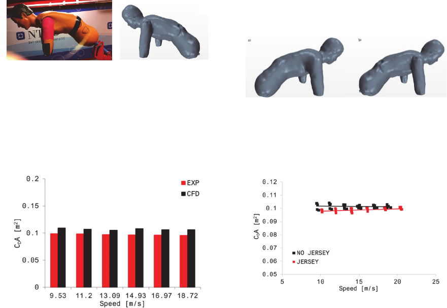
4.1.1 Validation Against Experiments

(Jersey on)

Figure 3: Mannequin model in the wind tunnel (left) and

3D laser scanned model (right).

Table 1: Comparison between experiments and

simulations for the mannequin with jersey on.

Figure 4: C

A values at different speeds for the

mannequin with the jersey on for experiments (red) and

simulations (black).

The results show that CFD simulations

consistently match experiments at different wind

speeds with an error between simulations and

experiments in the order of 10% which can

considered to be a good agreement (Blocken et al.,

2013). The results clearly show that the C

parameter is constant at different wind speeds

allowing further simulations to limited to a single

speed.

4.1.2 Effect of Jersey on the Surface

Two different configurations of the model were

simulated (with and without jersey) in order to

evaluate how the jersey could influence the overall

drag. The test was carried out at 14.93m/s with the

assumption that the drag coefficient would be

constant at different wind speeds. Grooves and

irregularities due to joints and mannequin

construction were present on the model without

jersey while these surface irregularities were either

covered or smoothed in the scanned model with the

jersey on (see Figure 5). In particular bumps and

imperfections on the back and shoulder area can be

seen in the Figure 5b while these imperfections are

smoothed out in the model shown in Figure 5a

Figure 5: 3D scanned model a) model with jersey on. b)

model without jersey.

The measured drag from the mannequin without jersey

resulted to be higher than the measured drag from the

mannequin with jersey on Figure 6.

Figure 6: Experimental results from the mannequin test

with and without jersey.

The comparison between CFD and experiments

presented in Figure 7 shows the same trend seen in

Figure 6 and the main conclusion is that placing a

jersey on the model surface affects the flow around

reduces drag.

Speed [m/s] 9.53 11.2 13.09 14.93 16.97 18.72

CFD 0.109 0.107 0.105 0.108 0.106 0.106

] EXP 0.098 0.098 0.097 0.096 0.096 0.095

Error [%] 10.9 8.8 8.4 11.9 10.4 11.3

icSPORTS 2015 - International Congress on Sport Sciences Research and Technology Support

186

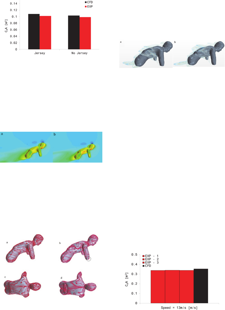
Figure 7: C

A values from experiments (red) and

simulations (black) for the mannequin model with and

without jersey at 14.93m/s.

The irregular surface on the plain model creates

low pressure zones that induce separation and

recirculation of the flow with a consequent increase

of pressure drag (Figure 8). In particular, it can be

seen in in Figure 8b the wake area is larger than in

Figure 8a. A high pressure area on the side of the

model without jersey is also present while the same

effect is not visible on the model with the jersey on.

Figure 8: Pressure contour plots on a) the mannequin with

jersey on and b) mannequin without jersey.

The same findings can be seen when plotting the

friction lines on the model. A recirculation area on

the side of the model can be seen. This recirculation

area is generated by the groove in the shoulder

region where the arm is attached to the torso. From

Figure 9 it can also be seen that the flow on the arm

separates differently on the model with jersey and on

the model without jersey.

Figure 9: Friciton lines on the model with jersey (a,c) and

without jersey (b,d).

Similar conclusions come also from figure 10

where the vorticity field around the model is

represented for visualization purposes. In the model

with no jersey Figure 10b, the groove in the shoulder

joint creates a vortex that develops and reattaches on

the side of the model while the irregularities in the

back induce separation.

Figure 10: Vorticity field around the mannequin model. a)

with jersey b) without jersey.

4.2 Cyclist

4.2.1 Validation Against Experiments

(Dropped Position)

Experiments were available only for the cyclist in

dropped position. The drag of the bare athlete with

no bike was obtained subtracting the drag measured

for the bare bike from the drag measurements from

the bike+cyclist test. While the experiments were

carried out at three different wind speeds, a single

CFD simulation at 13.09 m/s was carried out

assuming the C

A from CFD to be independent

from the wind speed.

The results from the CFD simulation match the

experiments with an error of 10% and the simulated

drag area C

A is consistently higher than the

measured one. The over prediction of the

aerodynamic drag is a known problem in CFD

simulations and it is directly linked to the turbulence

modelling (Blocken et al., 2013). The standard

turbulence models are in fact not able to correctly

simulate the vortices in the recirculation regions and

they often tend to keep the large structures without

correctly resolving the smaller structures that are

responsible of the vortex breaking mechanism,

leading to an over prediction of the total drag.

Figure 11: C

A values for the cyclist model from

simulations (black) and experiments (red).

Aerodynamical Resistance in Cycling - CFD Simulations and Comparison with Experiments

187

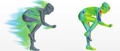
Figure 12 illustrates the vorticity field around the

cyclist and the pressure field on the cyclist. The

interaction between the different body parts can be

seen in Figure 12a where the vortices generated by

the arms directly interact with the athlete trunk.

Figure 12b gives an overview of the area where

separation might occur. The low pressure areas (blue

color) are areas where the flow is detached. Large

vortices are usually generated from these areas

leading to an increase in total drag. Major attention

to these areas is then important when designing a

low drag suit.

Figure 12: Vorticity field around the full model. And

pressure contour plots on the model.

5 CONCLUSIONS

CFD simulations proved to be a useful tool and the

results consistently matched the experimental results

with an over prediction estimated to be around 10%.

If on one side experiments are still needed,

especially for surface modifications and dynamic

testing, CFD could give a much better insight of the

pressure and force distribution on the body. CFD

could then be a good complementary tool to use in

parallel with wind tunnel testing

REFERENCES

Blocken, B., Defraeye, T., Koninckx, E., Carmeliet, J. &

Hespel, P. 2013. Cfd simulations of the aerodynamic

drag of two drafting cyclists. Computers & Fluids, 71,

435–445.

Brownlie, L. 1992. Aerodynamic characteristics of sports

apparel. Simon fraser university.

Brownlie, L., Gartshore, M., Mutch, B. & Banister, B.

1987. Influence of apparel on aerodynamic drag in

running. The Annals of Physiological Anthropology, 6,

133-143.

Brownlie, L., Kyle, C. R., Carbo, J., Demarest, N., Haber,

E., Macdonald, R. & Nordstrom, M. 2009.

Streamlining the time trial apparel of cyclists: the nike

swift spin project. Sports technology, 1-2, 53-60.

Cd-adapco 2015. Starccm+ user guide.

Chung, T. J. 2002. Computational fluid dynamics,

Cambridge University Press.

De Groot, G., Sargeant, A. & Geysel, J. 1995. Air friction

and rolling resistance during cycling. Medicine and

science in sports and exercise, 27, 1090–1095.

Debraux, P., Grappe, F., Manolova, A. V. & Bertucci, W.

2012. Aerodynamic drag in cycling: methods of

assessment. Sports biomechanics, 10, 197–218.

Defraeye, T., Blocken, B., Koninckx, E., Hespel, P. &

Carmeliet, J. 2010a. Aerodynamic study of different

cyclist positions: CFD analysis and full-scale wind-

tunnel tests. . Journal of biomechanics, 43, 1262-1268.

Defraeye, T., Blocken, B., Koninckx, E., Hespel, P. &

carmeliet, j. 2010b. Computational fluid dynamics

analysis of cyclist aerodynamics: performance of

different turbulence-modelling and boundary-layer

modelling approaches. Journal of Biomechanics, 43,

2281-2287.

Defraeye, T., Blocken, B., Koninckx, E., Hespel, P. &

Carmeliet, J. 2011. Computational fluid dynamics

analysis of drag and convective heat transfer of

individual body segments for different cyclist

positions. Journal of Biomechanics, 44, 1695–701.

Di Prampero, P. E. 2000. Cycling on earth, in space and

on the moon. European Journal Applied of

Physiology, 82, 345–360.

Hanna, R. K. 2002. Can CFD make a performance

difference in sport? In: Haake SJ, E. (ed.) The

Engineering of Sport 4. Oxford: blackwell science.

Launder, B. E. & sharma, B. I. 1974. Application of the

energy dissipation model of turbulence to the

calculation of flow near a spinning disc. Letters in

Heat and Mass Transfer, 1, 131-138.

Lecrivain, G., Slaouti, A., Payton, C. & Kennedy, I. 2008.

Using reverse engineering and computational fluid

dynamics to investigate a lower arm amputee

swimmer’s performance. Journal of Biomechanics, 13,

2855–2859.

Lukes, R. A., S.B., C. & S.J, H. 2002. The understanding

and development of cycling aerodynamics. Sports

engineering, 8, 59–74.

Menter, F. R. 1994. Two-equation eddy-viscosity

turbulence models for engineering applications. Aiaa

journa, 32, 1598–1605.

Minetti, A. E., Machtsiras, G. & C., M. J. 2009. The

optimum finger spacing in human swimming. Journal

of biomechanics, 42, 2188–90.

Oggiano, L. & Sætran, L. 2012. Experimental analysis on

parameters affecting drag force on speed skaters.

Sports technology, 3, 223-234.

Oggiano, L., Sætran, L., Leirdal, S. & Ettema, G. 2008.

Aerodynamic optimization and energy saving of

cycling postures for international elite level cyclists.

The Engineeeing of Sport 7, 597-604.

Oggiano, L., Troynikov, O., Konopov, I., Subic, A. & F.,

a. 2009. Aerodynamic behaviour of single sport jersey

fabrics with different roughness and cover factors.

Sports Engineering, 12, 1-12.

Spalart, P. R. 2000. Strategies for turbulence modelling

and simulations. Int. J. Heat Fluid Flow 21 (3), 252–

icSPORTS 2015 - International Congress on Sport Sciences Research and Technology Support

188

263.

Underwood, L. 2012. Aerodynamics of track cycling.

Doctor of philosophy, the University of Canterbury.

Underwood, L. & Jermy, M. C. Fabric testing for cycling

skinsuits. 5th Asia-pacific congress on sports

technology (APCST), 2011 Melbourne. 350–356.

Wilcox, D. C. 2006. Turbulence modelling for CFD, la

Canada, California, USA.

Zaïdi, H., Fohanno, S., Taïar, R. & Polidori, g. 2010.

Turbulence model choice for the calculation of drag

forces when using the CFD method. Journal of

Biomechanics, 10, 405-11.

Aerodynamical Resistance in Cycling - CFD Simulations and Comparison with Experiments

189