Genetic Algorithm as Machine Learning for Profiles Recognition

Yann Carbonne

and Christelle Jacob

University of Technology of Troyes, 12 rue Marie Curie, Troyes, France

Altran Technologies, 4 avenue Didier Daurat, Blagnac, France

Keywords: Genetic Algorithm, Machine Learning, Natural Language Processing, Profiles Recognition, Clustering.

Abstract: Persons are often asked to provide information about themselves. These data are very heterogeneous and

result in as many “profiles” as contexts. Sorting a large amount of profiles from different contexts and

assigning them back to a specific individual is quite a difficult problem. Semantic processing and machine

learning are key tools to achieve this goal. This paper describes a framework to address this issue by means

of concepts and algorithms selected from different Artificial Intelligence fields. Indeed, a Vector Space Model

is customized to first transpose semantic information into a mathematical model. Then, this model goes

through a Genetic Algorithm (GA) which is used as a supervised learning algorithm for training a computer

to determine how much two profiles are similar. Amongst the GAs, this study introduces a new reproduction

method (Best Together), and compare it to some usual ones (Wheel, Binary Tournament).This paper also

evaluates the accuracy of the GAs predictions for profiles clustering with the computation of a similarity

score, as well as its ability to classify two profiles are similar or non-similar. We believe that the overall

methodology can be used for any kind of sources using profiles and, more generally, for similar data

recognition.

1 INTRODUCTION

For several years, we have witnessed the exponential

growth of data worldwide. According to the experts,

90% of world data had been generated over the last

two years. Human cannot handle this large amount of

data, hence machine comes in the foreground for

processing and extracting meaningful information

from them.

In this paper, we will focus on a special kind of

data: those concerning people. These data can be very

heterogeneous due to the diversity of their origin.

Data comes from several sources: public (social

media, forums, etc.) or private (employee database,

customer database, etc.).

Despite their diversity, collected data are

processed the same way: each user (a real person) is

matched with one or several profiles. A profile could

contain global information (city, gender …) or

specific information (work history …). The

information volume could also be dense or sparse.

This paper differs from existing studies about

profiles recognition in social networks (Rawashdeh &

Ralescu, 2014) because it does not focus on similarity

between profiles within a social network but between

different social networks. Even if existing solutions,

such as the use of Vector Space Models (VSM) for

information retrieval (Salton, 1968), inspired our

study, they are not straight related.

The problem is to identify the same real person

between different profiles from different sources.

To do so, the objective is to teach a computer to

automatically answer the question: “Are these two

profiles about the same real person?”. Just like it

would be for a human, the teaching will be split in

two phases. During a first phase, the computer will

use a human-made set of data to train. Within this

training set, for each possible combination of profiles,

the question above had been answered. The training

should be done with various profiles from different

sources to be relevant. After the training phase, the

computer will be able to predict a similarity score

between two profiles. The performances will be

determined through the analysis of predefined criteria

for predictions.

In this study, we investigate how to determine a

person profile using a combination of natural

language processing, genetic algorithm and machine

learning. In addition, we propose a new reproduction

mechanism, named here Best Together (BT). The

Carbonne, Y. and Jacob, C..

Genetic Algorithm as Machine Learning for Proﬁles Recognition.

In Proceedings of the 7th International Joint Conference on Computational Intelligence (IJCCI 2015) - Volume 1: ECTA, pages 157-166

ISBN: 978-989-758-157-1

157

new reproduction is compared with other methods

such as Wheel and Binary Tournament. Results

indicate BT as a promising strategy for profile

recognition.

This paper is organized as follows: Section 2

introduces how to convert a profile (a set of semantic

information) to a mathematic model, understandable

for a computer. Section 3 describes the overview of

the genetic algorithm used to train the computer for

profile recognition. Section 4 analyses the results of

the prediction made by our model and it will be

followed by our conclusions.

2 MATHEMATICS DESIGN FOR

PROFILES

2.1 Representation of a Profile

First of all, let us introduce the mathematical model

used for profiles representation. A profile will be

considered as a set of labelled semantic information.

For example:

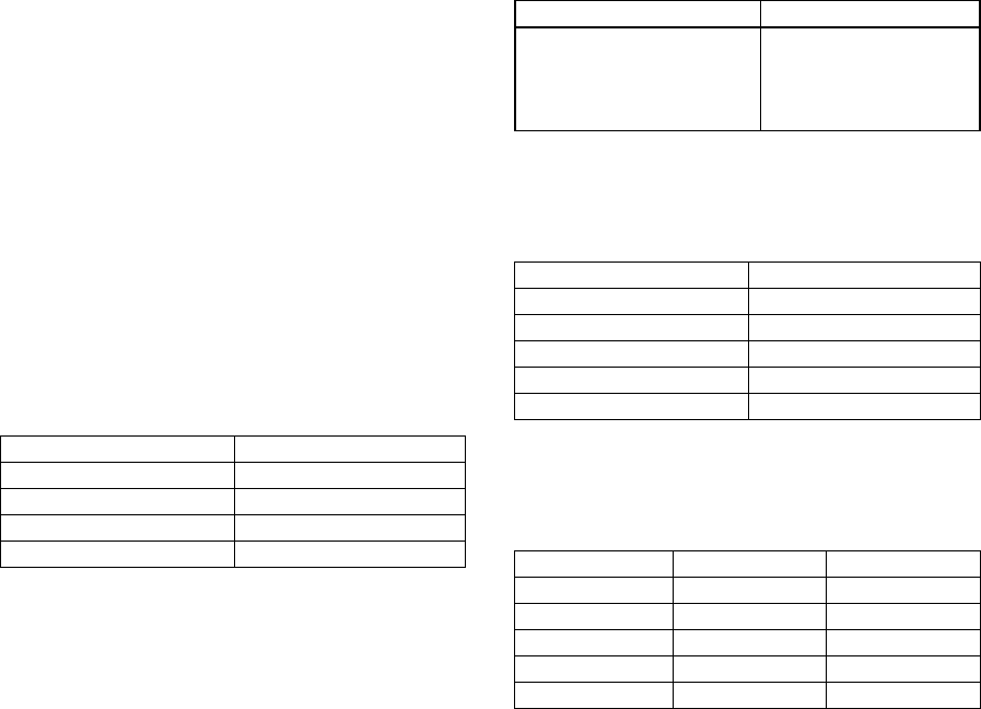
Table 1: Profile example.

Information Label

Foo firstname

Bar lastname

Paris city

beer like

In order to be able to compare several profiles on

a same frame of references, we will use the Vector

Space Models (VSM) of semantics.

Indeed, computers have difficulty understanding

semantic information but VSM provides a solution

for this problem. They have widely been used in

different fields as a recent survey highlights (Turney

and Pantel, 2010). In particular, they have been

successfully used in the field of Machine Learning for

classification (Dasarathy, 1991) and also for

clustering (A. K. Jain, 1999).

Within a VSM, each profile P

will be transposed

as a vector V

with N

dimensions which are all the

information in the profile P

. For example, the profile

above will be a vector with the dimensions: “Foo”,

“Bar”, “Paris” and “beer”.

The value of V

in a specific dimension δ will be

a weighting from the label matched with the

information δ.

The VSM consists in creating a new vector space

of M dimensions. For two vectors V

and V

, the

dimension M is set as:

M = N

∪ N

(1)

Whenever transposing a vector into a VSM, the

vector has a value 0 on its non-existing dimensions.

Illustration to the use of VSM with an example :

considering two profiles P

and P

Table 2: Contents for profiles P

and P

Foo firstname Foo firstname

Bar lastname Bar lastname

Google organisation Horses like

Paris city Google like

For the purpose of this example, the weighting for

each label are:

Table 3: Weighting example.

Label Weight

firstname 0.7

lastname 0.8

organisation 0.4

city 0.5

like 0.1

The associated VSM, with the vector V

for P

and

for P

, will be:

Table 4: VSM for V

and V

Dimension V

Foo 0.7 0.7

Bar 0.8 0.8

Google 0.4 0.1

Paris 0.5 0

Horses 0 0.1

The advantage of this representation is to keep the

semantic information in the forefront of the

mathematic analysis. In the example above, both

profiles have the information “Google” but for one,

this information is labelled as “organisation” and for

the other, it is labelled as “like”. Even with these

different labels, this model will consider the

information important but at a different scale. By

intuition, we would like to set the label “organisation”

at a higher value than the label “like” because the

former is usually more relevant to distinct two

profiles than the later. We acquired this intuition

through our experience and we would like the

computer to get the same “intuition” for any kind of

labels.

ECTA 2015 - 7th International Conference on Evolutionary Computation Theory and Applications

158

2.2 Similarity Function

Once the VSM for two vectors V

and V

is created,

the usual method is to compute their similarity with

the cosine (Turney and Pantel, 2010):

similarity (V

) = cos (α) (2)

where α is the angle between V

and V

This similarity rate gives a good clue of how close

two vectors are within their vector space, therefore

how similar two profiles are.

But there is a human intuition in profiles

recognition that is missing with this computation.

Sometimes, two profiles do not contain enough

relevant information to evaluate their similarity. For

example, if two profiles like the same singer and these

profiles only contain this information, it is not enough

to determine they both concern the same person.

Through experimentation, we noticed that the norm

of a vector is a good metric to evaluate the relevance

of a profile. Therefore, the similarity rate is smoothed

with the average norm of the two vectors:

similarity(V

) = cos(α) * (‖V

‖ + ‖V

‖) / 2

(3)

where ‖V‖ is the Euclidean norm for the vector V. The

factor (‖V

‖ + ‖V

‖) / 2 goes through a repair function

which assures it stays in the real interval [0,1].

This similarity rate is a real value in [0,1] and it

can be interpreted as a percentage. For example, a rate

of 0.27 corresponds to 27% of similarity.

To sum it up, making use a VSM is an effective

process to move from semantic information to a

mathematic model which will be used to compute

effectively the similarity between two profiles. The

next step is to teach the computer to find dynamically

the weighting for each label. For this purpose, a

genetic algorithm is applied in this study.

3 GENETIC ALGORITHM

Genetic algorithms (GA) are heuristics, based on

Charles Darwin’s theory of natural evolution, used to

solve optimization problems (Hüe, 1997). The

general process for a GA is described as follows

(Eberhart et al., 1996), (Kim and Cho, 2000):

Step 1: Initialize a population.

Step 2: Compute the fitness function for each

chromosome in the population.

Step 3: Reproduce chromosomes, based on their

fitness.

Step 4 : Perfom crossover and mutation.

Step 5 : Go back to step 2 or stop according to a

given stopping criteria.

GA can also be used as Machine Learning (ML)

algorithm and has been shown to be efficient in this

purpose (Goldberg, 1989). The idea behind is that

natural-like algorithms can demonstrate, in some

cases in the ML field, a higher efficiency compared

to human-designed algorithms (Kluwer Academic

Publishers, 2001). Indeed, actual evolutionary

processes have succeeded to solve highly complex

problems, as proved through probabilistic arguments

(Moorhead and Kaplan, 1967).

In our case, GA will be used to determine an

adequate set of weighting for each label present in a

training set. Our training set is composed with

similarities between profiles, two profiles are either

similar (output = 1) or not similar (output = 0).

3.1 Genetic Representation

The genotype for each chromosome of the population

will be the group of all labels in the training set. Each

label is defined as a gene and the weighting for a

specific label is the allele of the linked gene. The

weighting is a value in [0,1], it could be translated as

the relevance of a label and it reaches its best at value

1 and worst at 0.

3.2 Population Initialization

For population initialization, there are two questions

: “What is the initial population size ?” and “What is

the procedure to initialize the population ?”.

About the population size, the goal is to find a

compromise between the global complexity and the

performance of the solution (Holland, 1992). A small

population may fail to converge and a large one may

demand an excessive amount of memory and

computation time. It turns out that the size of the

initial population has to be carefully chosen, tailored

to address our specific problem.

As a reminder, in our problem, the GA have to

compute weighting for a number N of labels in the

training set. We evaluated different values for the

population size, compromised between efficienty and

complexity and chose to fix the population size to

2×N.

Secondly, to initialize a population, there are

usually two ways: heuristic initialization or random

initialization. The heuristic initialization, even if it

allows to converge faster to a solution, has the issue

to restrain the GA to search solutions in a specific area

and it may fail to converge to a global optimum (Hüe,

1997). A random initialization is a facilitating factor

for preventing GA to get stuck in a local optima.

In our case, the random initialization consists in

Genetic Algorithm as Machine Learning for Proﬁles Recognition

159

giving a random weighting between [0,1] for each

gene within the genotype.

3.3 Fitness Function

The main purpose of a fitness function is to evaluate

a chromosome, based on how well it fits the desired

solution (Hüe, 1997).

In our case, chromosomes are evaluated on how

well they fit the training set, using the VSM method

to predict similarities. We chose to use a fitness

function which is widely used in the ML field (Shen,

2005), as our problem can be related to a regression

problem. It is called the logarithmic loss which is

defined as follows:

loss= -

(y

log

i=1







1- y



log(1- p

))

(4)

where M is the number of examples in our training

set, y

is the output (0 or 1) of the ith example and p

is the output in [0;1] from the current chromosome.

To prevent the asymptote at 0 from the logarithmic

function, the predicted output p is replaced with:

p:maxmin



p,1‐10

‐15



,10

‐15



(5)

3.4 Crossover

Crossover is the artificial reproduction method for a

GA. It has to define how two selected chromosomes

will produce an offspring. Crossover is crucial for

GA, causing a structured exchange of genetic

information between solutions which could lead good

solutions to better ones (Srinivas and Patnaik, 1994).

We chose to use the arithmetic crossover with an

alpha parameter at 0.5. This crossover creates

children that are the weighted arithmetic mean of two

parents:

offspring = 0.5 * parent1 + 0.5 * parent2 (6)

3.5 Mutation

Mutation forces some chromosomes to change and it

allows the GA to get away from a local optima (Hüe,

1997).

In our case, the risk to get stuck in a local optima

is present. Indeed, the aim for our GA is to find the

optimized weighting for a set of labels which consists

in finding the relevant labels (high weighting) and the

non-relevant ones (low weighting), consequently

creating an ordering for the labels. Local optima

would consists of a version of the GA detecting that,

for example, the label “lastname” is relevant to find

some similarities within the training set. This result

will lead to a better fitness function. But it would be

a local optima due to the necessity to find the right

weighting and ranking for each label. The GA should

be defined with a sufficient amount of diversity which

will allows keeping a good weighting for a specific

label but still enabling variation to the other labels.

Therefore, we chose to implement a mutation

method which enhances the diversity.

Beside the mutation chance M

, which determines

the chance for an offspring to mutate, we set up a

mutation rate M

. If a new chromosome mutates (i.e.

if a random number in [0,1] < M

), each of its alleles

will vary depending on a random factor F in [1 - M

1 + M

]. Of course, a repair function is applied to

ensure that each allele stays in [0,1].

3.6 Reproduction

The reproduction (or selection) method is intended to

improve the average quality for a new generation. To

fulfill this goal, this method usually follows the

Darwin’s principle that the fittest chromosomes will

tend to reproduce more (Hüe, 1997).

There are two categories of reproduction methods:

proportionate and ordinal-based.

The first one is based on the fitness value and

gives each chromosome a chance to reproduce

proportionally to its value. A typical method is the

wheel (Goldberg, 1989). We consider a wheel where

each chromosome has a portion with a size

proportional to its score. To select partners for

crossover, we simply “launch” the wheel. With this

method, each chromosome has a chance to be a

parent, even so, statistically, the fittest chromosomes

might have a better chance than the others.

On the contrary, for ordinal-based methods, the

chromosomes are ranked according to their fitness

and the selection is based upon the rank of a

chromosome within the population. A classical

approach is the use of the tournament method (Miller

and Goldberg, 1995). This method needs to get a

parameter S (tournament size) which determines the

size for a round. In fact, this method proceeds round

after round. At each round, S chromosomes are

randomly selected, the highest-ranked chromosome

wins the round and it is selected for crossover.

However, for this specific problem of profiles

recognition, we came up with a new idea which will

be presented afterwards. Then, we will show the

results in comparison with the state of the art of

reproduction method.

Usually, a GA have a low mutation chance (~

0.05) which leads to a controlled diversity. The

ECTA 2015 - 7th International Conference on Evolutionary Computation Theory and Applications

160

reproduction method also controls the diversity by

letting globally a chance for each chromosome to be

selected for crossover.

The idea of our GA is to set up a huge mutation

factor (Section 3.5) which will ensure the diversity of

our algorithm and prevent it to get stuck in a local

optima. Beside this point, the tactic is to have a highly

selective reproduction method which allows to get rid

of all non-adequate chromosomes. To sum up, a

generation will have a lot of diversity but will quickly

throw non-suitable chromosomes away. The diversity

is assured by our mutation method, so we just need

the reproduction method to be selective.

Consequently, we created our own reproduction

method, labelled as Best Together (BT). It is inspired

by the idea of considering only an elite group of

chromosomes for reproduction, introduced with the

incoming of Biased Random-Key Genetic

Algorithms (Resende, 2010). It is an ordinal-based

method; thereby it is necessary to rank the population.

For a population of size N, this method will select a

number X of the best chromosomes. Each of these

selected chromosomes will reproduce with all others

selected chromosomes. We know that it leads to a

number of crossover equals to:

X * (X – 1) / 2

(7)

Each crossover producing an offspring, the

population size needs to stay approximately the same.

To do so, we need the equation 7 to be equal to N,

which leads to the following polynomial equation:

X² - X – 2*N = 0 (8)

The X computed by the BT method is the positive

solution of this quadratic form (which always exists

because if a = 1 and c = -2, then the determinant ≥ 0).

The solution might be a real number, therefore only

the floor of X is kept. It slightly decreases the

population size but it does not really affect the quality

of the GA.

As we explained, once the BT method has

computed this value X, it takes a group of X best

chromosomes and applies crossover with all

combinations, except for a chromosome with itself.

3.7 Comparison

In (Section 3.6), we presented a new reproduction

method which differs from the state of the art. In this

section, we will compare it with some state of the art

GA over our training set.

We compared 3 GA with the following

parameters:

1) A wheel reproduction.

2) A tournament reproduction with a

tournament size 2 (binary tournament).

3) Our BT reproduction method.

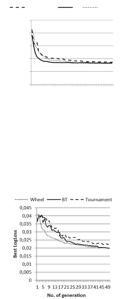
For the figure 1, we set M

= 0.75 and M

= 0.8, which

is considered as a large mutation chance and we saved

the best score for the fitness function in each

generation.

Figure 1: Comparison of reproduction with a large

mutation.

The BT method converges faster than the Wheel and

Tournament methods: it reaches a LogLoss value

below 0.17 at the 14

generation. The Wheel reaches

this threshold at the 27

generation and the

Tournament does not reach it within the first 50

generations.

But the BT method is a specific method for a large

mutation chance and it performs poorly with a low

mutation chance. As you can observe with the figure

2, where we set M

= 0.1 and M

= 0.8:

Figure 2: Comparison of reproduction with a low mutation.

0,01

0,02

0,03

0,04

0,05

1 5 9 13 17 21 25 29 33 37 41 45 49

BestLogLoss

No.ofgeneration

Tournament BT Wheel

Genetic Algorithm as Machine Learning for Proﬁles Recognition

161

4 RESULTS

The real test of our algorithm will be done in a

supervised machine learning context. It will be

evaluated for the quality of its predictions.

For that, we trained our model with the GA

presented in (Section 3) over a training set composed

of 3,003 similarities between profiles. In the training

set, an output for a similarity between two profiles is

either 1 (the two profiles correspond to the same

person) or 0. Apart from the training set, we have a

test set, composed with 741 similarities and their

output with the same format. This set is not used to

train the model with the GA; its only purpose is to

evaluate predictions for our trained model.

These sets are extracted from different sources.

Therefore, each set is really disparate because its

contain profiles with different size.

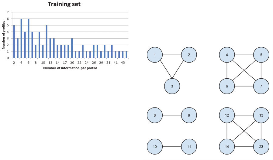
Figure 3: Distribution of the profiles in the training set.

The distribution of profiles, in the training set,

according to the number of information per profile is

as follows:

Within the training set, the average information

per profile is 14.49 but the standard deviation is

11.13. This standard deviation is really high

compared with the average, which proves the

diversity in the training set. Even if the test set is

smaller, its average is 14.57 and its standard deviation

is 11.08, which is almost the same diversity as the

training set.

During our training phase, our model learns from

a dataset with discrete outputs. But as we are using a

mathematical model (described in section 2) based on

cosine to compute similarity rate, the outputs are

continuous values.

Therefore, this section will present how our model

performs on this test set viewed from two aspects:

regression problem and classification. The former

will evaluate our original model to predict continuous

valued output, corresponding to the similarity rate

between two profiles. The second will adapt our

model to determine if either two profiles are similar

(class = 1) or non-similar (class = 0).

4.1 Regression Problem

In our case, the regression problem is translated into

the capacity for our model to determine that some pair

of profiles are more similar than others, even if all

these pairs correspond to the same person (output =

1). The differences between similarity rates come

from the fact that, even for a human, deducing that 2

profiles correspond to the same person is more

obvious with some data than others.

But we cannot objectively evaluate the similarity

score computed by our model. Imagine that, for a

specific pair of profiles, our model sets up a similarity

score at 0.7. As humans, a value of 0.7 has no

meaning when it comes to decide whether two

profiles concern the same person, or two. We expect

“yes” or “no”. For our model, 0.7 makes sense from

a computational point of view.

Actually, what we really need is to find clusters of

profiles which correspond to the same person.

In our test set, we have the following clusters:

Figure 4: Clusters within the test set.

Each node represents a profile and each link

represents a similarity between 2 profiles (output =

1). The cluster 1 – 2 – 3 means that each profile is

related to the same real person.

Our model predicted the following clusters:

ECTA 2015 - 7th International Conference on Evolutionary Computation Theory and Applications

162

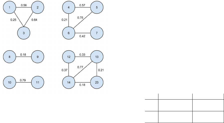
Figure 5: Clusters prediction.

Each value matched with a link corresponds to a

similarity value between 2 profiles. We removed the

links with a 0 value.

The first observation is that each cluster is there,

even if some links (5-7, 4-7 and 12-23) are missing.

This means that the model allows us to indirectly link

profiles which are not similar with the direct

comparison of their data.

We can also observe an expected pattern with the

first cluster (1-2-3), where the links 1-2 and 2-3 have

strong similarities while the link 1-3 is weak. Indeed,

when we look closer at the test set, the profile 2

contains more relevant information than both profiles

1 and 3. Therefore, this is really positive that our

model is also able to detect both strong and weak

similarities.

4.2 Binary Classification

For binary classification, we need our model to be

able to classify two profiles as similar (class 1,

positive class) or non-similar (class 0, negative class).

4.2.1 Threshold

In order to allow our model to classify two profiles,

we need to set up a threshold. Two profiles with a

predicted value below this threshold will be classified

as the class 0, otherwise as the class 1.

As part of the learning phase, this threshold shall

be tuned so as to match user’s expectation about the

model. A high threshold should be used if the user

wants his model to be restrictive to determine that two

profiles are similar and, in return, a low threshold for

an extendible model is needed.

To give an example, in the context of our project,

we fixed the threshold to 0.075 because we presume

that two profiles are similar when some relevant

information match.

4.2.2 Metrics

First of all, we need to define the different metrics

widely used in binary classification problems.

In binary classification, a model predicts if a data

has a class 0 or 1 (predicted class) and a dataset

indicate the actual class for this data.

Then, we can introduce 4 metrics as follow:

Table 5: Main metrics for binary classification.

Actual Class

1 0

Predicted

Class

1 True positive False

positive

0 False

negative

True

negative

In general, positive = identified and negative =

rejected. Therefore:

 True positive (TP) = correctly identified

 False positive (FP) = incorrectly identified

 True negative (TN) = correctly rejected

 False negative (FN) = incorrectly rejected

Usually, a metric accuracy is used and defined as:

 



 





⁄

(9)

where M = size of the dataset.

But in our case it will not be relevant because we

can define our class 1 as a skewed class. Our training

set is composed with 3003 similarities but only 26 of

them (0.87%) have an output of 1. It means that if a

model predicts always the class 0, it would have an

accuracy of 99.13%.

Therefore, a binary classification problem with a

skewed class is defined as an imbalanced learning

problem and it should be handled specially (He &

Garcia, 2009). Then, we would use other metrics such

as precision (P) and recall (R). Precision is defined as

follows:

     

⁄

(10)

This metrics is useful to evaluate how well a

model predicts positives values.

The recall (R) is defined as follows:

    

⁄

(11)

This metric, also named sensitivity, measures the

rate of a model to predict incorrect positives classes.

Genetic Algorithm as Machine Learning for Proﬁles Recognition

163

These two metrics are really useful but there is an

issue: they are interdependent.

Supposing that we want the model to predict that

two profiles are similar only if it is very confident (i.e.

avoid false positives). Then, we would fix the

threshold to a high value, like 0.9. Doing so, the

model will have a higher precision and a lower recall.

On the contrary, considering we would like a

model which avoid missing similarities between

profiles (i.e. avoid false negatives). This time, we

would fix the threshold to a low value, like 0.1. The

result will be a higher recall and a lower precision.

Now, the problem is that we need a good metric

that will help to find a balance between precision and

recall. As an illustration, considering the following

table:

Table 6: Use of Average to compare Precision and Recall.

Precision Recall Average

0.5 0.4 0.45

0.7 0.1 0.4

0.02 1.0 0.51

Genuinely, the first pair (0.5, 0.4) seems better

than the last pair (0.02, 1.0) which is unbalanced. But

the first pair has a worse average than the last pair.

To prevent that, we introduce a last metric, the F1-

Score, as follows:

12 

⁄

(12)

This metric is a weighted average of the precision and

recall and we will use this one to measure our test

accuracy.

To show its effectiveness, we updated the table

above with this new metric:

Table 7: Comparison of the Average and F1Score.

Precision Recall Average F1Score

0.5 0.4 0.45 0.444

0.7 0.1 0.4 0.175

0.02 1.0 0.51 0.0392

The F1Score, as well as the other metrics, reaches

its best at value 1 and worst score at 0.

For our test set, we tried different values for the

threshold:

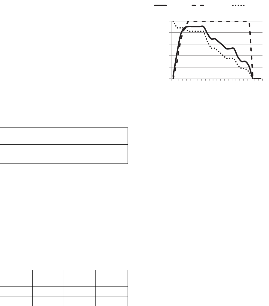
Figure 6: Precision, Recall and F1Score within the test set.

Considering this figure, the first information is that

our model is highly precise. From a low threshold

(0.075) to the highest prediction within the test set

(0.79), the metric precision is always at 1. This level

of precision allows to select a low threshold. This low

threshold also permits to keep a high value for the

metric recall, which gets lower when the threshold

rises.

4.2.3 ROC Curve

In binary classification, a Receiver Operation

Characteristic (ROC) curve is a statistical tool for

evaluating a classifier and choosing a threshold. In

particular, it is fundamental in medicine to determine

a cutoff value for a clinical test (Campbell & Zweig,

1993).

The curve is created by plotting the true positive

rate in function of the false positive rate at various

threshold settings. In Machine Learning, the true

positive rate is the metric called recall and the false

positive rate is named fall-out. The fall-out is defined

as follows:



      

⁄

(13)

A high threshold would decrease both fall-out and

recall. However, the objective is to get the highest

recall and the lowest fall-out. Indeed, a test with

perfect discrimination has a ROC curve that passes

through the point (0,1) which is called a perfect

classification. Therefore, the closer the curve is to the

upper left corner, the higher the overall accuracy of

the test (Campbell & Zweig, 1993).

The graphical plot of the ROC curve for our test

set is as follows:

0,025

0,075

0,125

0,175

0,25

0,35

0,45

0,55

0,65

0,75

0,85

0,2

0,4

0,6

0,8

Threshold

Value

F1Score Precision Recall

ECTA 2015 - 7th International Conference on Evolutionary Computation Theory and Applications

164

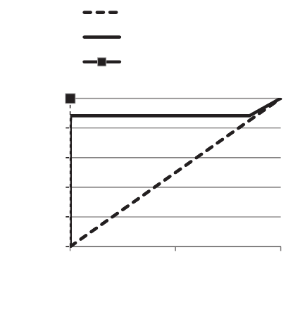
Figure 7: ROC curve within the test set.

The linear line from the point (0,0) to the point (1,1)

corresponds to a random classification and is called

the line of no-discrimination.

The elbow of the curve (i.e. the best trade-off

point) is explicit and correspond to our selected

threshold of 0.75. The curve for our classifier is really

close to the perfect classification which proves the

high accuracy of our model.

5 CONCLUDING REMARKS

In this paper, we proposed and developed a machine

learning algorithm based on a genetic algorithm for

profiles recognition. Our solution is a combination

between natural language processing, evolutionary

algorithm and surpervised machine learning.

First, we recalled how to represent a profile in a

Vector Space Models, in order to ease the processing

of semantic data.

In a second part, the principle of genetic

algorithms is described; and used to train the

computer to evaluate the significance of each label.

This phase still requires human intervention throught

a training set.

Finally, we tested the model predictions within a

complete new dataset. These predictions revealed a

highly precise model.

Our model allowed to automatically determine

both a similarity score between profiles and which

profiles correspond to the same person.

The solution proposed in this paper is adaptable

and generic. This adaptation is due to the fact that the

model is not restricted to a fixed set of labels. As long

as the labels are present into the training set, both the

mathematical model and the genetic algorithm would

adapt to a new set of labels.

Therefore we strongly believe it could be used for

any kind of sources containing profiles. Moreover,

this solution could also be used to other applications

of similar data recognition.

ACKNOWLEDGEMENTS

We are thankful to Michel Bordry for his help during

the manuscript review. We also thank Andréa

Duhamel for her insightful comments.

REFERENCES

A. K. Jain, M. M. P. F., 1999. Data Clustering: A Review.

ACM Computing Surveys (CSUR), Volume 31, pp. 264-

323.

Campbell, G. & Zweig, M. H., 1993. Receiver-Operation

Characteristic (ROC) Plots: A Fundamental Evaluation

Tool in Clinical Medicine. Clin Chem, 39(4), pp. 561-

577.

Dasarathy, B. V., 1991. Neared neighbor (NN) Norms: NN

Pattern Classification Techniques. IEEE Computer

Society Press.

Eberhart, R. C., Simpson, P. K. & Dobbins, R., 1996.

Computational Intelligence PC Tools. s.l.:AP

Professional.

Goldberg, D. E., 1989. Genetic Algorithms in Search,

Optimization, and Machine Learning. Boston, MA,

USA: Addison-Wesley Longman Publishing Co., Inc.

He, H. & Garcia, E. A., 2009. Learning from Imbalanced

Data. IEEE Transactions on Knowledge and Data

Engineering, Volume 21, pp. 1263-1284.

Holland, J. H., 1992. Adaptation in natural and artificial

systems. Cambridge, MA, USA: MIT Press.

Hüe, X., 1997. Genetic Algorithms for Optimisation :

Background and Applications. s.l.:s.n.

Kim, H. & Cho, S., 2000. Application of interactive genetic

algorithm to fashion design. Engineering Applications

of ArtiÆcial Intelligence.

Kluwer Academic Publishers, 2001. Genetic Algorithms

and Machine Learning. Machine Learning.

Miller, B. L. & Goldberg, D. E., 1995. Genetic Algorithms,

Tournament Selection, and the Effects of Noise.

Complex Systems, Issue 9, pp. 193-212.

Moorhead, P. S. & Kaplan, M. M., 1967. Mathematical

challenges to the neo-Darwinian interpretation of

evolution. Wistar institute symposium monograph,

Issue 5.

Rawashdeh, A. & Ralescu, A. L., 2014. Similarity Measure

for Social Networks - A Brief Survey.

Resende, M. G., 2010. Biased Random-key genetic

00,51

0,2

0,4

0,6

0,8

FallOut

Recall

RandomClassification

OurClassification

PerfectClassification

Genetic Algorithm as Machine Learning for Proﬁles Recognition

165

algorithms with applications in telecommunications.

AT&T Labs Research Technical Report.

Salton, G., 1968. Automatic Information Organization and

Retrieval.

Shen, Y., 2005. Loss Functions for Binary Classification

and Class Probability Estimation, s.l.: University of

Pennsylvania.

Srinivas, M. & Patnaik, L. M., 1994. Adaptive Probabilities

of Crossover and Mutation in Genetic Algorithms.

IEEE Transactions on systems, man and cybernetics,

Volume 24, pp. 656-667.

Turney, P. D. & Pantel, P., 2010. From Frequency to

Meaning : Vector Space Models of Semantics. Journal

of Artificial Intelligence Research.

ECTA 2015 - 7th International Conference on Evolutionary Computation Theory and Applications

166