Weighting and Sampling Data for Individual Classiﬁers and Bagging

with Genetic Algorithms

so Karakati

c, Marjan Heri

cko and Vili Podgorelec

Institute of Informatics, UM FERI, Smetanova 17, Maribor, Slovenia

Keywords:

Classiﬁcation, Genetic Algorithm, Instance Selection, Weighting, Bagging.

Abstract:

An imbalanced or inappropriate dataset can have a negative inﬂuence in classiﬁcation model training. In

this paper we present an evolutionary method that effectively weights or samples the tuples from the train-

ing dataset and tries to minimize the negative effects from innaprotirate datasets. The genetic algorithm with

genotype of real numbers is used to evolve the weights or occurrence number for each learning tuple in the

dataset. This technique is used with individual classiﬁers and in combination with the ensemble technique of

bagging, where multiple classiﬁcation models work together in a classiﬁcation process. We present two vari-

ations – weighting the tuples and sampling the classiﬁcation tuples. Both variations are experimentally tested

in combination with individual classiﬁers (C4.5 and Naive Bayes methods) and in combination with bagging

ensemble. Results show that both variations are promising techniques, as they produced better classiﬁcation

models than methods without weighting or sampling, which is also supported with statistical analysis.

1 INTRODUCTION

Supervised machine learning methods, such as classi-

ﬁcation, use a process of learning where a computer

is presented with a set of solved tuples (classiﬁcation

instances with known results). This set is called a

train dataset and its purpose is to help with classi-

ﬁcation model creation. The quality of the resulting

machine learning model is heavily dependent on the

tuples from the train dataset, where a proper train set

helps with the creation of a good model, but inappro-

priate train tuples can misguide the learning algorithm

and prevent it from reaching the optimal solutions.

Inappropriate train datasets can harm the model

creation in following ways (Stefanowski and Wilk,

2008), (Japkowicz and Stephen, 2002):

• Mislabeled tuples. Mislabeling can be a result of

a human or machine error and force the learning

process to result in false conclusions. The model

is then built upon a false presentation of reality

and does not perform well on real problems.

• Imbalanced datasets. The nature of machine

learning algorithms is such that they learn in a

way that minimizes the errors. Over representa-

tion of a certain class of individuals can harm this

process. More speciﬁcally, big differences in fre-

quencies of classes can cause the algorithm to in-

tentionally ignore or under-emphasize the minori-

ties.

• Outliers. Outliers are individuals that are not nec-

essary in a minority class but are nonetheless low

in frequency in certain properties. This situation

where some attributes of individuals are heavily

outnumbered can cause algorithms to ignore some

important aspects of the dataset or misinterpret it

for an error.

Several techniques exist which can help to over-

come the problem of inappropriate train dataset. First

body of techniques is gathered under an umbrella

term of instance selection methods (Liu, 2010). The

theory of instance selection methods postulates that

we can select some individuals from original train

dataset that are then used to train the model. There

are numerous variations on how the training subset is

selected.

Another approach to solve the problem is with the

use of ensemble methods (Dietterich, 2000), where

multiple classiﬁcation models cooperate together to

form a ﬁnal solution. But again all classiﬁers in the

ensemble are prone to (although to a lesser extent)

error based on the inappropriate train datasets.

We propose a novel method to solve this problem

of inappropriate train datasets, which can be used by

any individual classiﬁer or in combination with en-

180

Karakati

c, S., Heri

cko, M. and Podgorelec, V..

Weighting and Sampling Data for Individual Classiﬁers and Bagging with Genetic Algorithms.

In Proceedings of the 7th International Joint Conference on Computational Intelligence (IJCCI 2015) - Volume 1: ECTA, pages 180-187

ISBN: 978-989-758-157-1

semble method bagging. Our method is applied in

the pre-processing part of learning process and uses a

genetic algorithm to construct the train dataset by ei-

ther subsample and oversample, or weighing the clas-

siﬁcation tuples. Two interesting variations arise and

are presented this paper: sampling the train data and

weighting the train data. The proposed method is

tested on individual classiﬁers as with bagging en-

semble method, to determine the effectiveness and

potential usefulness of the method.

The rest of the paper is constructed as follows.

The second section takes an overview of related work

from the body of relevant literature of instance selec-

tion and train dataset preparation. Next, the third sec-

tion presents the genetic algorithm that is used in our

method. Multiple variations of the genetic algorithm

are presented: for individual classiﬁers, for ensem-

bles, with sampling and with weighting. Fourth sec-

tion is dedicated to the experiments with our method

and its variations where we make comparisons with

traditional classiﬁcation methods and ensemble tech-

niques, to determine the quality of our method. After

that we conclude the paper with a discussion of results

and possible future development on the subject.

2 RELATED WORK

There have been numerous studies done on rebalanc-

ing the datasets with the goal of achieving better ﬁnal

outcomes of classiﬁcation. Most of these are done

with instance selection from the datasets, where the

method of selections generates the subset of original

dataset and then uses it in classiﬁcation model. For a

good overview of these methods refer to a survey on

tuple selection methods (Olvera-L

opez et al., 2010).

Selection methods are divided in categories:

• Wrapper methods. These methods use the classi-

ﬁcation metrics to determine which tuples should

be selected for ﬁnal subset of tuples. Usual metric

used here is overall classiﬁcation accuracy.

• Filter methods. This method uses some other met-

ric or function that is not based on the classiﬁca-

tion results.

Our method of sampling and weighting is a wrap-

per approach as it uses classiﬁcation accuracy as a

metric for selection. Next we follow up with the re-

view of relevant literature on wrapper methods, espe-

cially in combination with evolutionary methods.

Main tuple selection approaches are based on

the nearest neighbor (NN) methods, such as con-

densed NN (Angiulli, 2005), selective NN (Linden-

baum et al., 2004) and generalized condensed NN

(Chou et al., 2006). These methods use a method of

ﬁnding the nearest neighbors to remove the unwanted

tuples that are either too similar to one and another or

by removing dense clusters of tuples from the dataset.

An extension of regular NN methods are IB2 and IB3

algorithms, that incrementally removes or preserves

missclassiﬁed tuples by 1-NN algorithm (Wilson and

Martinez, 2000).

Evolutionary algorithms have also been used

for the tuple selection wrapper methods. There

are numerous methods based on genetic algo-

rithms (Kuncheva and Bezdek, 1998), (Bezdek and

Kuncheva, 2001) and (Cano et al., 2003). All of these

methods use an array of 0 and 1 in arrays, where

each gene represents the absence (0) or presence (1)

of each classiﬁcation tuple. As described later in

section 3 this genotype representation is very simi-

lar to our approach, but we extend this by allowing

genes to have integers larger then 1, thus not just se-

lecting a tuple but effectively sampling data with re-

placements. Our method uses the same genetic op-

erators as have been used in this literature, as our

goal was to present novel genotype representation and

not to ﬁnd optimal operator settings. One interest-

ing method used genetic algorithms in combination

with neural networks to select optimal subset of orig-

inal train dataset (Kim, 2006). In another paper re-

searchers used genetic algorithm for feature and tuple

selection (Tsai et al., 2013), but used GA to determine

which method should they use. Another combination

of kNN method and GA is used in a paper (Garca-

Pedrajas and Prez-Rodrguez, 2012).

The problem with these selection methods is

that they only remove individuals from the original

dataset, but they do not repeat instance occurrence in

the dataset it this would provide any additional im-

provements. Tuple selection technique can thus be de-

ﬁned as an undersampling method, but research show

that random undersampling (removing tuples on ran-

dom) (Kotsiantis and Pintelas, 2003) can lead to in-

formation loss and consequently to less than optimal

classiﬁcation models (Japkowicz, 2000), (Japkowicz

and Stephen, 2002), (Kubat and Matwin, 1997). In a

paper (Cateni et al., 2014) researchers use a combi-

nation of undersampling the majorities and oversam-

pling the minority tuples to achieve an equilibrium

and improved classiﬁcation. Oversampling and un-

dersampling at the same time is usually called sam-

pling dataset with replacements, where an algorithm

selects desired number of tuples and they can repeat

in the new dataset.

Sampling with replacements (or even without

them) is used in some ensemble methods, such as bag-

ging (Breiman, 1996), where a chosen amount of new

Weighting and Sampling Data for Individual Classiﬁers and Bagging with Genetic Algorithms

181

datasets are sampled from the original train dataset.

Each of these new datasets is then used as a train set

for a classiﬁcation method. Each classiﬁer then pro-

duces a slightly different model which then partici-

pates in an ensemble. The ﬁnal decision of an en-

semble is determined by a majority vote from all of

the models in an ensemble. In it’s original form, the

bagging method selects bags (sampled datasets) by

simple uniform random fashion. Later in section 4

we also use our method in combination with the bag-

ging method. Our contribution to the ﬁeld is that our

method also builds the bags in a such way, that the

whole ensemble is more efﬁcient in basic classiﬁca-

tion metrics.

Weighting tuples is a similar process to sampling,

but instead of duplicating or removing tuples we as-

sign weights to them, where a higher weight implies

a higher importance and a lower weight denotes less

important tuples. Weighting tuples is done in boosting

algorithms, such as AdaBoost (Freund et al., 1996).

We can reproduce weighting in sampling form, where

the ratio between weights is the same as the ration be-

tween the frequency of tuple occurrence. This is done

in combination with methods that cannot work with

weighted datasets. Nonetheless, weighting is prefer-

able to sampling because it uses less computation re-

sources (no redundant computation necessary for du-

plicated tuples). Weighting tuples have also been

done in (Zhao, 2008), (Ting, 2002), (Liu et al., 2013),

(Liu and Yu, 2007) and (Cano et al., 2013). We also

use weights in tuples in one variation of our method,

but the main difference from sampling method is not

ratio, but the weight and frequency distribution, as

will be presented in the next section.

3 GENETIC ALGORITHMS FOR

WEIGHTING AND SAMPLING

Genetic algorithm (GA) is a method in the ﬁeld of

evolutionary computation and can be used on vari-

ous optimization problems. GA mimics the process

of evolution and natural selection where population

is guided with ﬁtness functions to its ﬁnal goal. It

has been proposed by Holland in his work Adaptation

in Natural and Artiﬁcial System (Holland, 1992) and

many variations have been made since then.

Population in GA is a set of individuals where

each individual represents the solution to a given

problem. In our case we dealt with the sampling and

weighting of train dataset, so the genotype of one in-

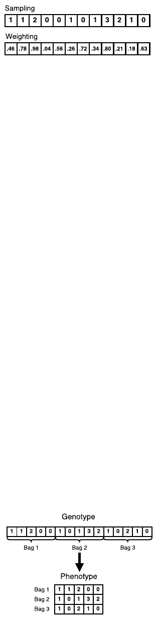
dividual is constructed from an array of numbers (see

ﬁgure 1). Each gene is linked with one tuple from the

train dataset. Gene with index of i represents a tuple

Figure 1: Top – array genotype for sampling variation. Each

gene value represents the occurrence number for each tuple.

Bottom – array genotype for weighting variation. Each gene

value represents the weight for each tuple.

with index i from the dataset. Here we are given two

options on how to construct our genotype. In the case

of sampling we can use an array of integers where

each gene shows the number of occurrences of a given

tuple from the dataset. The default case without sam-

pling would be the array of all genes set to 1, as each

tuple is in our dataset once. When gene value is set

to 0 that tuple is not present in a train set and does

not play a role in training of a classiﬁcation model.

Naturally the genes can have integers higher than 1,

meaning that tuples are duplicated so their number is

the same as the value of its gene. The initialization of

this type of genotype is done as the random number

from the set with normal distribution with the mean

on 1 and the standard deviation as the changing pa-

rameter. Note that example occurrences in the dataset

can not be set as the negative number, which means

that random executes again until the resulting number

is valid.

The second option of individuals representation

is for weighting tuples, where genotype is an array

of real numbers where the numbers are weights as

shown in ﬁgure 1. Weights in gene say how much

importance is given to it’s linked tuple – the higher

the number, more important is that particular tuple.

Again, if any given gene has a value set to zero weight

it means that it does not participate in the training of

the model. The real difference from the previously

described genotype is with the initialization of the

genes. Each weight (gene value) is randomly chosen

from the set of number in [0, 1] in an uniform distri-

bution.

These two variations of the genotype are also used

in a combination with the bagging method. With bag-

Figure 2: Genotype and phenotype for bagging method.

ECTA 2015 - 7th International Conference on Evolutionary Computation Theory and Applications

182

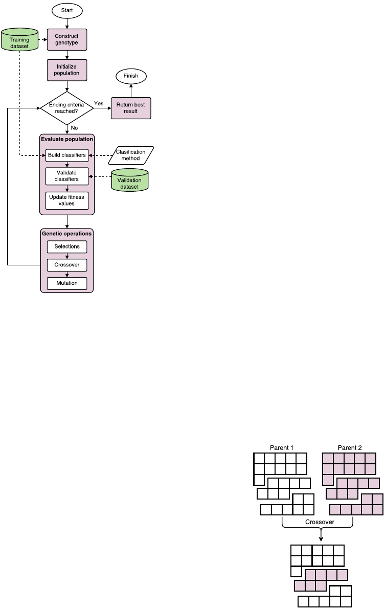
Figure 3: Flowchart of the whole evolutionary process.

Note that Classiﬁcation method presents an algorithm for

building classiﬁcation model.

ging we have multiple different sets (bags), which can

overlap or be disjointed. The extensions of genotypes

for bagging is such that the array is repeated for each

bag. Figure 2 presents the genotype and its transfor-

mation to the phenotype (note that only sampling vari-

ation is shown in the ﬁgure, but the representation is

the same for weighting in bagging).

The basic ﬂowchart of GA methods is depicted in

ﬁgure 3 and goes as follows. First the initial popula-

tion is generated – each individual solution is made

in the process described previously. Then we eval-

uate each individual solution with the ﬁtness func-

tion. Calculating the ﬁtness levels starts with build-

ing a classiﬁcation model with a chosen classiﬁca-

tion method on sampled or weighted train dataset and

evaluating it on the validation dataset. Classiﬁcation

metric error rate of the built model is used as the ﬁt-

ness value, which means that the ﬁtness function tries

to minimize it’s value and ideally hit zero.

After the evaluation the selection process starts.

Here we use a standard binary tournament method

which randomly chooses two individual solutions

from the population and selects the one with a bet-

ter value. Selected solutions are then paired and go

through a genetic operator of crossover, where both

parent solutions contribute a part of their genotype

to form a new child solution. The ordered crossover

(OX) is used, also known as a two-point crossover.

Here, two points between genes are selected, same in

both parents, and the part between two points are ex-

changed. This results in two offspring solutions that

continue through the process of evolution. This kind

of crossover is used in a combination with individ-

ual classiﬁers or with bagging. As ﬁgure 4 shows,

some bags are copied whole, but some bags can be cut

and can include genes from both parents. This forces

changing of individual bags and not only combination

of bags, which would be the case if only whole bags

were mixed in the crossover process.

The resulting children have a small chance to go

through a genetic operator of mutation, where one

gene is randomly selected and it’s value is changed

to a random value with the same method as is used

for the creation of the genotypes. When the mutation

is ﬁnished, children solutions then form a new popu-

lation and form a basis for the next generation.

4 EXPERIMENTS

In this section we present the results of our experi-

ments. All four variations of our method have been

used in the experiments:

• Sampling for single classiﬁers

• Weighting for single classiﬁers

• Sampling for Bagging

• Weighting for Bagging

These methods were tested in combination with

traditional classiﬁcation methods: C4.5 (Quinlan,

1993) and Naive Bayes (John and Langley, 1995).

Figure 4: Ordered crossover for bagging ensemble. Some

bags can be cut in two parts – this forces evolution of indi-

vidual bags, as well as mixing of different bags.

Weighting and Sampling Data for Individual Classiﬁers and Bagging with Genetic Algorithms

183

Our method was also compared to models trained on

original datasets and on bagging.

We used 11 standard classiﬁcation benchmark

datasets from UCI repository (Lichman, 2013), which

have been divided in the following way: 60% for

training, 20% for validation and 20% for testing. The

datasets were split in a random fashion and this pro-

cess was repeated 5 times, in order to minimize the

possibility for false conclusions. This is similar to us-

ing 5 fold cross validation, but instead of using 4 fold

for training and 1 fold for testing, we used 3 folds for

training, 1 for validation and 1 for testing. Same splits

(folds) were used on all of the methods, to insure en-

sure the comparability of the results.

The settings for genetic algorithm were as fol-

lows: 100% chance of ordered crossover, 10% chance

of random exchange mutation, population of 100 in-

dividual, 200 generations and binary tournament se-

lection. The bagging method used an ensemble of

5 classiﬁcation models (5 bags). The genetic algo-

rithm and experimental setup were programmed in

Java programming language and used in combination

with Weka machine learning framework.

4.1 Spread of Sampling

In the ﬁrst experiment we tried to determine whether

there are any signiﬁcant differences in models when

initialization process of genes uses a different stan-

dard deviation for random generator based on normal

distribution. The experiment was made with bagging

and base classiﬁer C4.5 and the use of sampling vari-

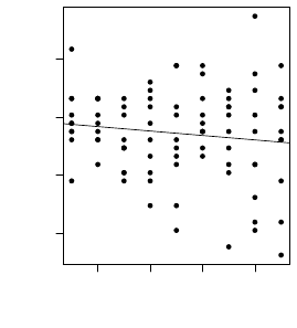
ation of our method. In ﬁgure 5 we see a liner regres-

sion model where we look at the accuracy metric.

1 2 3 4

0.65 0.70 0.75 0.80

Standard deviation

Overall classification accuracy

Figure 5: Trend of changing standard deviation in the ini-

tialization of genes for sampling variation.

The slope of the trend line indicates a slight de-

cline in the overall accuracy as standard deviation in-

creases, but is enough that we use standard deviation

of 1 for further experiments as it produces ac-

curate and least volatile results.

4.2 Experiments with Traditional

Classiﬁcation Methods

Here we compare our method with the traditional

classiﬁcation methods in combination with both sam-

pling and weighting. In table 1 we see the resulting

accuracy and average F-score of C4.5 method. All

of the results are averaged on all of the folds, which

is standard in a cross-validation process. We ﬁrst

identiﬁed the distribution type of the results and then

continued with the appropriate tests. None of the re-

sults had normal distribution (both Shapiro-Wilk and

Kolmogorov-Smirnov tests return p < 0.05) so we

used non-parametric tests for the comparison. First

Friedman’s Two-Way ANOVA was used to determine

if there are signiﬁcant differences between all com-

pared groups. If ANOVA conﬁrmed the differences,

we continued with post-hoc where we used Wilcoxon

signed-rank test (non-parametric alternative to t-test

for related samples) and Holm-Bonferroni correction

(correction for multiple comparison to reduce the

chance of a Type I error).

There are differences in accuracies between the

methods, but these differences are not statistically

signiﬁcant as shown by the Friedman’s Two-Way

ANOVA for related samples (p

acc

= 0.120). On

the other hand the differences in the F-scores have

reached statistical signiﬁcance (p

f sc

= 0.011). Post-

hoc test with the Holm-Bonferonni correction show

that there are statistically signiﬁcant differences be-

tween C4.5 and sampling with C4.5 (p = 0.008), while

differences C4.5 vs weighting and weighting vs sam-

pling are not signiﬁcant (p = 0.110 and p = 0.674 re-

spectively). Based on the presented results (the me-

dian value and the Friedman ranks) we can conclude

that our two variation are at least as good and can even

be better as C4.5 without our methods.

Next we made the same experiment with Naive

Bayes methods and results are shown in table 2. In all

but two datasets our methods achieved better results in

comparison to classiﬁer without sampling or weight-

ing. In one case (iris dataset) the results were tied.

Although there are no statistically signiﬁcant differ-

ences in either of the metric (p

acc

= 0.154 and p

f sc

= 0.115) we can see a trend in the resulting metrics.

Best median value and the highest Friedman rank was

achieved by sampling method in both metrics.

ECTA 2015 - 7th International Conference on Evolutionary Computation Theory and Applications

184

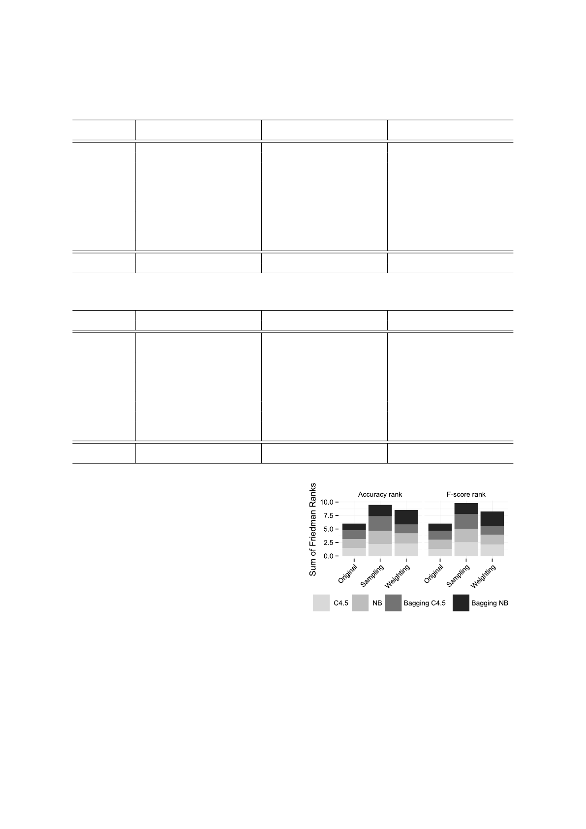
Table 1: Accuracy and F-score results on all benchmarks for C4.5 and two variations of our method with C4.5. Accuracies

are averaged across folds. Bolded values show the best results for given metric in particular dataset.

C4.5 Sampling Weighting

Accuracy F-score Accuracy F-score Accuracy F-score

autos 0,7343 0,7278 0,7829 0,7786 0,7229 0,7107

balance-scale 0,7714 0,7514 0,7590 0,7533 0,7829 0,7533

breast-cancer 0,7104 0,6764 0,7292 0,7111 0,7167 0,6889

car 0,9003 0,8992 0,9038 0,9052 0,8788 0,8755

credit-a 0,8391 0,8393 0,8400 0,8399 0,8609 0,8608

diabetes 0,7227 0,7140 0,7359 0,7349 0,7398 0,7321

heart-c 0,7510 0,7471 0,7569 0,7555 0,7843 0,7828

heart-statlog 0,7667 0,7645 0,7800 0,7795 0,8022 0,7995

iris 0,9320 0,9320 0,9440 0,9437 0,9360 0,9360

primary-tumor 0,3982 0,3462 0,3982 0,3749 0,3807 0,3144

vehicle 0,7177 0,7124 0,7156 0,7124 0,7241 0,7194

Median 0.7510 0.7471 0.7590 0.7555 0.7829 0.7533

Friedman Rank 1.50 1.32 2.23 2.55 2.27 2.14

Table 2: Accuracy and F-score results on all benchmarks for Naive Bayes and two variations of our method with Naive Bayes.

Accuracies are averaged across folds. Bolded values show the best results for given metric in particular dataset.

Naive Bayes Sampling Weighting

Accuracy F-score Accuracy F-score Accuracy F-score

autos 0.5486 0.5470 0.5743 0.5586 0.5857 0.5731

balance-scale 0.8857 0.8462 0.8886 0.8558 0.8886 0.8514

breast-cancer 0.7208 0.7094 0.7229 0.7150 0.7125 0.6939

car 0.8378 0.8256 0.8604 0.8519 0.8806 0.8712

credit-a 0.7704 0.7612 0.8070 0.8031 0.8061 0.8012

diabetes 0.7383 0.7350 0.7422 0.7368 0.7633 0.7575

heart-c 0.8412 0.8404 0.8627 0.8625 0.8373 0.8367

heart-statlog 0.8533 0.8526 0.8489 0.8481 0.8467 0.8464

iris 0.9520 0.9519 0.9520 0.9519 0.9520 0.9512

primary-tumor 0.4754 0.4411 0.4614 0.4148 0.4474 0.4016

vehicle 0.4298 0.3868 0.5184 0.5049 0.4858 0.4634

Median 0.7704 0.7612 0.8070 0.8031 0.8061 0.8012

Friedman Rank 1.64 1.68 2.41 2.50 1.95 1.82

4.3 Experiments with Bagging

Ensemble

In this section we present the results of the experi-

ments on the bagging ensemble method. Again we

used 11 benchmark sets from the previous experi-

ment. Experiments with bagging were repeated on

the previously used classiﬁcation methods: C4.5 and

Naive Bayes. The results where we again aggregated

the resulting metrics from all folds in the same value.

In table 3 the results for bagging with C4.5 are

presented. The statistical analysis shows that there

are signiﬁcant differences in the accuracy and aver-

age F-score (p

acc

= 0.013 ; p

f sc

= 0.013). In post-

hoc test for accuracy we see that sampling variation

is superior to both the basic bagging and the sam-

pling method (for both p = 0.022). The results for

F-score are similar – the sampling method resulted in

superior solutions when compared to both, weighting

and basic methods (both p = 0.022). Table 4 presents

Figure 6: Comparing sum of Friedman’s Ranks. Higher is

better.

the results for bagging with Naive Bayes base classi-

ﬁer and we can see that our method (both variations)

achieve better results in all ten datasets. Statistical

tests (Friedman’s ANOVA) shows that there are sig-

niﬁcant differences in both metrics (p

acc

= 0.002 ; p

f sc

= 0.012). Further post-hoc tests (Wilcoxon signed-

Weighting and Sampling Data for Individual Classiﬁers and Bagging with Genetic Algorithms

185

Table 3: Accuracy and F-score results on all benchmarks datasets for Bagging with base classiﬁer C4.5. Comparison between

our two variations with Bagging (C4.5) and default bagging without sampling or weighting. Accuracies are averaged across

folds. Bolded values show the best results for given metric in particular dataset.

Bagging with C4.5 Sampling Weighting

Accuracy F-score Accuracy F-score Accuracy F-score

autos 0.7343 0.7276 0.8086 0.6886 0.8075 0.6691

balance-scale 0.7971 0.7817 0.8048 0.8229 0.7874 0.7881

breast-cancer 0.7000 0.6613 0.7375 0.7208 0.7062 0.6806

car 0.9090 0.9086 0.9382 0.8972 0.9387 0.8905

credit-a 0.8513 0.8507 0.8504 0.8652 0.8499 0.8651

diabetes 0.7305 0.7259 0.7344 0.7438 0.7279 0.7382

heart-c 0.7706 0.7691 0.7745 0.7765 0.7732 0.7746

heart-statlog 0.7933 0.7914 0.7800 0.8156 0.7772 0.8136

iris 0.9640 0.9638 0.9680 0.9440 0.9679 0.9439

primary-tumor 0.3860 0.3514 0.4140 0.4281 0.3819 0.3549

vehicle

0.7220 0.7167 0.7504 0.7241 0.7461 0.7166

Median 0.7706 0.7691 0.7800 0.7765 0.7772 0.7746

Friedman Rank 1.64 1.64 2.73 2.73 1.64 1.64

Table 4: Accuracy and F-score results on all benchmarks datasets for Bagging with base classiﬁer Naive Bayes. Comparison

between our two variations with Bagging (Naive Bayes) and default bagging without sampling or weighting. Accuracies are

averaged across folds. Bolded values show the best results for given metric in particular dataset.

Bagging with Naive Bayes Sampling Weighting

Accuracy F-score Accuracy F-score Accuracy F-score

autos 0.5686 0.5550 0.6057 0.5928 0.6000 0.5880

balance-scale 0.8857 0.8465 0.8933 0.8537 0.8990 0.8590

breast-cancer 0.7250 0.7190 0.7292 0.7146 0.7354 0.7255

car 0.8413 0.8297 0.8535 0.8433 0.8587 0.8473

credit-a 0.7757 0.7668 0.7817 0.7740 0.8017 0.7961

diabetes 0.7500 0.7423 0.7516 0.7451 0.7594 0.7550

heart-c 0.8333 0.8330 0.8353 0.8352 0.8510 0.8496

heart-statlog 0.8333 0.8321 0.8311 0.8297 0.8356 0.8344

iris 0.9480 0.9476 0.9400 0.9394 0.9640 0.9638

primary-tumor 0.4807 0.4424 0.4842 0.4460 0.4807 0.4256

vehicle 0.4390 0.3952 0.4965 0.4688 0.4504 0.4115

Median 0.7757 0.7668 0.7817 0.7740 0.8017 0.7961

Friedman Rank 1.23 1.36 2.09 2.00 2.68 2.64

rank test with Holm-Bonferroni correction) for accu-

racies reveal that the signiﬁcant differences exist be-

tween our weighting method and the basic method (p

= 0.002), while differences between the basic method

and sampling variation are not signiﬁcant (p = 0.086).

The same post-hoc analysis was done for the F-score

metric and again there are statistical signiﬁcant differ-

ences between the basic bagging (with Naive Bayes)

and our weighting method (p = 0.006).

5 CONCLUSIONS

We presented an evolutionary method for manipu-

lating the training dataset in two variations with the

hopes of producing better classiﬁcation models. Both

variations are based on genetic algorithm where the

genotype represents the number of occurrences or

weights of any particular tuple. We can conclude,

based on the results, that our methods for individual

classiﬁers of sampling and weighting can produce re-

sults that are at least as good (and in some cases bet-

ter) as the method without them. In the metrics we

see improvements, but these differences are mostly

not statistically signiﬁcant. On the other hand, our

methods for bagging produce major improvements on

both metrics and these improvements are signiﬁcant,

which means that our genetic algorithm indeed helps

with the construction of better models. In ﬁgure 6 we

compare sum of the ranks of all variations included

in the experiment. The higher sum indicates better

results in different conditions (with different classi-

ﬁers). The sampling variation has the highest sum of

ranks and is followed by weighting variation of our

method. This indicates that the sampling variation is

superior to weighting and to original (no sampling nor

weighting) in context of our experiment. Further ex-

ECTA 2015 - 7th International Conference on Evolutionary Computation Theory and Applications

186

amination of the sum of ranks reveals that the weight-

ing variation was still preferred in combination with

bagging and Naive Bayes. This means that there is

no universally best variation – as it is expected in the

ﬁeld of classiﬁcation, where universally best classiﬁer

cannot exist.

Further work will include using our methods with

more classiﬁcation algorithms, to determine what

kind of algorithms work better with sampling or

weighting and how to choose appropriate variation.

Future work could also include the usage of other

metrics for evaluation in our ﬁtness function.

REFERENCES

Angiulli, F. (2005). Fast condensed nearest neighbor rule.

In Proceedings of the 22Nd International Conference

on Machine Learning, ICML ’05, pages 25–32, New

York, NY, USA. ACM.

Bezdek, J. C. and Kuncheva, L. I. (2001). Nearest proto-

type classiﬁer designs: An experimental study. Inter-

national Journal of Intelligent Systems, 16(12):1445–

1473.

Breiman, L. (1996). Bagging predictors. Machine learning,

24(2):123–140.

Cano, A., Zafra, A., and Ventura, S. (2013). Weighted data

gravitation classiﬁcation for standard and imbalanced

data. Cybernetics, IEEE Transactions on, 43(6):1672–

1687.

Cano, J. R., Herrera, F., and Lozano, M. (2003). Using

evolutionary algorithms as instance selection for data

reduction in kdd: an experimental study. Evolutionary

Computation, IEEE Transactions on, 7(6):561–575.

Cateni, S., Colla, V., and Vannucci, M. (2014). A method

for resampling imbalanced datasets in binary classiﬁ-

cation tasks for real-world problems. Neurocomput-

ing, 135(0):32 – 41.

Chou, C.-H., Kuo, B.-H., and Chang, F. (2006). The gen-

eralized condensed nearest neighbor rule as a data re-

duction method. In Pattern Recognition, 2006. ICPR

2006. 18th International Conference on, volume 2,

pages 556–559. IEEE.

Dietterich, T. G. (2000). Ensemble methods in machine

learning. In Multiple classiﬁer systems, pages 1–15.

Springer.

Freund, Y., Schapire, R. E., et al. (1996). Experiments with

a new boosting algorithm. In ICML, volume 96, pages

148–156.

Garca-Pedrajas, N. and Prez-Rodrguez, J. (2012). Multi-

selection of instances: A straightforward way to im-

prove evolutionary instance selection. Applied Soft

Computing, 12(11):3590 – 3602.

Holland, J. H. (1992). Adaptation in natural and artiﬁcial

systems: an introductory analysis with applications to

biology, control, and artiﬁcial intelligence. MIT press.

Japkowicz, N. (2000). The class imbalance problem: Sig-

niﬁcance and strategies. In Proc. of the Intl Conf. on

Artiﬁcial Intelligence. Citeseer.

Japkowicz, N. and Stephen, S. (2002). The class imbalance

problem: A systematic study intelligent data analysis.

John, G. H. and Langley, P. (1995). Estimating continuous

distributions in bayesian classiﬁers. In Proceedings

of the Eleventh conference on Uncertainty in artiﬁcial

intelligence, pages 338–345. Morgan Kaufmann Pub-

lishers Inc.

Kim, K.-j. (2006). Artiﬁcial neural networks with evo-

lutionary instance selection for ﬁnancial forecasting.

Expert Systems with Applications, 30(3):519–526.

Kotsiantis, S. and Pintelas, P. (2003). Mixture of expert

agents for handling imbalanced data sets. Annals of

Mathematics, Computing & Teleinformatics, 1(1):46–

55.

Kubat, M. and Matwin, S. (1997). Addressing the curse of

imbalanced data sets: One sided sampling. In Proc. of

the Int’l Conf. on Machine Learning.

Kuncheva, L. I. and Bezdek, J. C. (1998). Nearest proto-

type classiﬁcation: clustering, genetic algorithms, or

random search? Systems, Man, and Cybernetics, Part

C: Applications and Reviews, IEEE Transactions on,

28(1):160–164.

Lichman, M. (2013). UCI machine learning repository.

Lindenbaum, M., Markovitch, S., and Rusakov, D. (2004).

Selective sampling for nearest neighbor classiﬁers.

Machine learning, 54(2):125–152.

Liu, H. (2010). Instance selection and construction for data

mining. Springer-Verlag.

Liu, J.-F. and Yu, D.-R. (2007). A weighted rough set

method to address the class imbalance problem. In

Machine Learning and Cybernetics, 2007 Interna-

tional Conference on, volume 7, pages 3693–3698.

Liu, X.-Y., Li, Q.-Q., and Zhou, Z.-H. (2013). Learning

imbalanced multi-class data with optimal dichotomy

weights. In Data Mining (ICDM), 2013 IEEE 13th

International Conference on, pages 478–487.

Olvera-L

opez, J. A., Carrasco-Ochoa, J. A., Mart

ınez-

Trinidad, J. F., and Kittler, J. (2010). A review of

instance selection methods. Artiﬁcial Intelligence Re-

view, 34(2):133–143.

Quinlan, J. R. (1993). C4.5: programs for machine learn-

ing. Elsevier.

Stefanowski, J. and Wilk, S. (2008). Selective pre-

processing of imbalanced data for improving classi-

ﬁcation performance. In Song, I.-Y., Eder, J., and

Nguyen, T., editors, Data Warehousing and Knowl-

edge Discovery, volume 5182 of Lecture Notes in

Computer Science, pages 283–292. Springer Berlin

Heidelberg.

Ting, K. M. (2002). An instance-weighting method to in-

duce cost-sensitive trees. Knowledge and Data Engi-

neering, IEEE Transactions on, 14(3):659–665.

Tsai, C.-F., Eberle, W., and Chu, C.-Y. (2013). Ge-

netic algorithms in feature and instance selection.

Knowledge-Based Systems, 39(0):240 – 247.

Wilson, D. R. and Martinez, T. R. (2000). Reduction tech-

niques for instance-based learning algorithms. Ma-

chine learning, 38(3):257–286.

Zhao, H. (2008). Instance weighting versus threshold ad-

justing for cost-sensitive classiﬁcation. Knowledge

and Information Systems, 15(3):321–334.

Weighting and Sampling Data for Individual Classiﬁers and Bagging with Genetic Algorithms

187