Cartesian Genetic Programming in a Changing Environment
Karel Slany
Department of Computer Systems, Faculty of Information Technology, Brno University of Technology,
Bo
ˇ
zet
ˇ
echova 2, 612 66, Brno, Czech Republic
Keywords:
Cartesian Genetic Programming, Age Layered Population Structure, Changing Environment.
Abstract:
Evolutionary algorithm are prevalently being used in static environments. In a dynamically changing environ-
ment an evolutionary algorithm must be also able to cope with the changes of the environment. This paper
describes an algorithm based on Cartesian Genetic Programming (CGP) that is used to design and optimise
a solution in a simulated symbolic regression problem in a changing environment. A modified version of the
Age-Layered Population Structure (ALPS) algorithm is being used in cooperation with CGP. It is shown that
the usage of ALPS can improve the performance on of CGP when solving problems in a changing environ-
ment.
1 INTRODUCTION
Cartesian Genetic Programming (CGP) was develo-
ped by J. Miller as a method for evolving digital cir-
cuits (Miller, 1999). Standard genetic programming
(GP) utilises a tree-like representation of a candidate
solution (Koza, 1992). By contrast, CGP genotypes
are represented with bounded oriented graphs. This
built-in limitation makes CGP suitable for running on
specialised embedded or resource-limited hardware.
The behaviour of CGP has been investigated from
different angles. The influence of aspects such as
modularity (Walker and Miller, 2005) or the use of va-
rious search strategies (Miller and Smith, 2006) have
been investigated. The influence of various mutation
operators and the usage of different pseudo-random
number generators have been presented (Va
ˇ
s
´
ı
ˇ
cek and
Sekanina, 2007).
The role of neutrality (Collins, 2006), (Yu and
Miller, 2001) has proven to be crucial especially when
solving difficult tasks. CGP contains a built-in me-
chanism of neutral mutation and a redundant geno-
type to phenotype mapping which improves the ef-
ficiency of searching in the fitness landscape (Ebner
et al., 2001). The existence of neutral networks helps
when changes in the environment occur.
A good evolutionary algorithm must also be able
to maintain population diversity. The algorithm
should be able to escape a local optima. A straight-
line solution is restarting the evolution with different
random seeds which increases the chances of finding
an optimal solution. A different approach is to period-
ically introduce new randomly generated individuals.
Such algorithm then has to ensure that the new indivi-
duals cannot be easily outperformed by solutions that
have been already present in the population.
This paper uses an already present combination
of CGP and a diversity maintaining algorithm. This
combination has already been presented on image fil-
ter evolution (Slan
´
y, 2009) where the algorithm was
able to find better solutions whereas the ordinary CGP
algorithm already stalled. However, the performance
of the algorithm in a changing environment has not
been investigated. This paper illustrates, using a syn-
thetic symbolic regression problem, that the algorithm
is more suitable for solving tasks in a changing envi-
ronment than the standard CGP evolutionary strategy.
2 CARTESIAN GENETIC
PROGRAMMING
In CGP a circuit (or programme) is represented
by an oriented acyclic graph organised into a two-
dimensional grid of nodes. The circuit has n
i
inputs
and n
o
outputs. The structure of CGP is depicted in
fig. 1.
Every node represents a primitive function from
the set primitive functions Γ. Every node is repre-
sented by a number of genes. The function gene f
i
204
Slany, K..
Cartesian Genetic Programming in a Changing Environment.
In Proceedings of the 7th International Joint Conference on Computational Intelligence (IJCCI 2015) - Volume 1: ECTA, pages 204-211
ISBN: 978-989-758-157-1
Copyright
c
 2015 by SCITEPRESS – Science and Technology Publications, Lda. All rights reserved

Figure 1: General form of a CGP genotype. The genotype
forms a grid of nodes which represent functions from the
set of primitive functions Γ. Each node takes as many in-
puts as the maximal function arity a. Data inputs and nodes
are numbered consequently. These numbers are then be-
ing used for addressing places where the input data or node
outputs can be accessed.
holds the address of a function in the function set for
the given node i. The connection genes c
i
hold the in-
formation about the location where the node i gets its
input from. Connection indexes are usually indexes
into an array of intermediate results. The indexes may
be relative (Harding, 2008) or absolute (Miller and
Thomson, 2000). The programme inputs are associ-
ated with addresses in the range starting with 0 and
ending at n
i
− 1.
The user selects the number of columns n
c
, the
number of rows n
r
and the level-back (or l-back) pa-
rameter l. Parameter l controls the interconnectivity
of the encoded graph. When l = 1 then each node can
take its input from the previous column. With l = n
c
each node can connect to any node in any preceding
column or any primary input. A special case of n
r
= 1
and l = n
c
is worth notice as it allows maximum level
of interconnectivity between the graph nodes.
The process of phenotype evaluation starts with
the identification of active nodes. These are recur-
sively identified by traversing the graph structure in
reverse – starting from the outputs. Nodes that have
not been identified as active are called non-coding.
Non-coding nodes are not processed during pheno-
type evaluation. The consequence of non-coding
nodes is that CGP phenotypes have variable size. The
size cannot exceed the size defined by the grid dimen-
sion n
c
× n
r
.
CGP uses mutation. Alleles at randomly chosen
gene locations are altered with another valid value.
Function genes can only be replaced with another
function gene values. Mutated connection genes must
obey the rules given for connection genes. The total
number of mutated genes is usually given by the per-
centage of the total number of genes in the genotype.
The value is called mutation rate µ
r
. Crossover oper-
ations are not commonly used in CGP.
CGP usually uses a simple evolutionary algorithm
known as (1+λ) evolutionary strategy where the best
individual is kept in the population. The number of
offspring is usually set to be a low number between 4
and 8. Suppose there is no better individual than the
parent but there are offspring with equal fitness to the
parent’s fitness. In that case the offspring is chosen
to be the new parent. The whole CGP algorithm is
summarised in alg. 1.
Algorithm 1: (1 + λ) Evolutionary Strategy.
g ← 0
for all i : 0 ≤ i < (1 +λ) do
pop[i] ← randomly generated individual
end for
Calculate the fitness for all individuals in population pop.
parent ← fittest individual from pop  pop[λ]
while (g < max number of generations) ∧ (fitness not acceptable) do
for all i : 0 ≤ i < λ do
pop[i] ← mutated parent  Offspring i.
end for
Calculate the fitness for all individuals in pop.
if some offspring fitness ≥ parent fitness then
parent ← offspring with equal or better fitness
end if
g ← g + 1  Increment generation counter.
end while
2.1 ALPS Algorithm
Premature convergence has been a problem in genetic
programming. It can be tackled by increasing the mu-
tation probability which will boost the diversity of the
population. But, increased mutation rate is very likely
to destroy good alleles which have already evolved
in the population. With mutation probability set high
the genetic algorithm cannot narrow the surroundings
of a particular solution. Large population sizes can
also solve the problem of reduced diversity at risk of
higher computational costs.
The Age-Layered Population Structure (ALPS)
(Hornby, 2006) introduces time labels into the evo-
lutionary algorithm. These labels represent the age
of particular candidate solutions. Individuals keep
the information about how long they have been evol-
ving. Candidate solutions are only allowed to interact
with individuals within the same age group. This en-
sures that newly generated solutions cannot be easily
outperformed by a solution which has already been
present in the population. Moreover, randomly ge-
nerated new solutions are added in regular intervals.
These principles are used to maintain population di-
versity in ALPS.
Newly generated solutions start with their respec-
tive age tag set to 0. Individuals generated by a ge-
netic operator, such as mutation or crossover, receive
the age of the oldest parent increased by 1. Also,
every time an individual is selected to be an parent,
its age is increased by 1. Should a candidate solu-
Cartesian Genetic Programming in a Changing Environment
205

tion be used as parent multiple times then its age is
increased by 1 only once.
The population is defined as a structure of age
layers which restrict the competition (and breeding)
among candidate solutions. Every layer except the top
layer has its age limit which restricts the residence of
candidate solutions to individuals with their age be-
low the value of the limit. The top layer has no age
restrictions. The structure of the layers can be de-
fined in various ways. Different systems are shown in
tab. 1. The factor values are multiplied by the age-gap
parameter. The product then serves as the maximal
age allowed in a particular layer.
Table 1: Ageing scheme distribution examples that can be
used in the ALPS algorithm.
ageing scheme limiting factor per layer
1 2 3 4 i
linear 1 2 3 4 i
polynomial 1 2 4 9 (i − 1)
2
,i > 2
exponential 1 2 4 8 2
i−1
factorial 1 2 6 24 i!
2.1.1 ALPS and CGP
Originally, ALPS was designed to maintain diversity
in difficult problems being solved by GP. GP uses a
crossover operator combined with tournament selec-
tion. The original algorithm has been modified so it
could operate with CGP (Slan
´
y, 2009). The modified
version utilises mutation and elitism. The crossover
operator has been removed.
The modified ALPS algorithm for CGP starts with
a randomly populated bottom layer. Layers above are
empty and are going to be filled during the evolution
process. The layers interact by sending offspring into
layers above or by receiving individuals from layers
below. The individuals grow older and are moved to
adjacent layers or are discarded. The bottom layer is
in regular intervals regenerated by randomly genera-
ted individuals with age 0. The parameter controlling
this behaviour is called randomisation-period. The
value of this parameter stands for the number of ge-
nerations between two adjacent randomisations of the
bottom layer.
Every time when the age of an individual exceeds
the age limit assigned to a given layer then such in-
dividual is moved to the next superordinate layer. If
there is a layer that should be populated by the off-
spring of its own and also by the offspring of a subor-
dinate layer then it is divided into two halves. The first
half is going to receive offspring from the layer itself.
The second half receives offspring from the layer be-
low. After this step, both halves become a single layer
again. Should a layer receive offspring only from a
layer below or only from itself then the entire layer
is going to be filled at once. The whole algorithm is
summarised in alg. 2.
Elitism similar to CGP is used. The best evolved
member is kept in each layer. It is replaced only
by individuals with better or at least equal fitness.
Should the algorithm omit the randomisation period
and should it use only a single layer then it would
equally match the (1 + λ) evolutionary strategy.
Algorithm 2: Modified ALPS algorithm for CGP.
g ← 0
l ← 0
for all i : 0 ≤ i < (1 +λ) do
pop[l][i] ← randomly generated individual
end for
Calculate the fitness for all individuals in population pop[l].
parent[l] ← fittest individual from pop[l]  pop[l][λ]
while (g < max number of generations) ∧ (fitness not acceptable) do
for all l : l
max
> l ≥ 0 do
if (0 = l) ∧ (0 = gmodrandom period) then
for all i : 0 ≤ i < (1 +λ) do  Randomise bottom layer.
pop[l][i] ← randomly generated individual
end for
else
auxp
this
← none
auxp
below
← none
mid ← 0
max ← 0
start
if (l = l
top
) ∨ (age(parent[l]) < age
max
(l)) then
auxp
this
← parent[l]  Parent in layer l.
mid ← (1 +λ)
end if
if (l 6= l
bottom
) ∧ (age(parent[l −1]) ≥ age
max
(l −1)) then
auxp
this
← parent[l −1]  Parent in layer l − 1.
if 0 6= mid then
mid ← (mid/2)
end if
max ← (1 + λ)
end if
if 0 6= mid then  Use parent from layer l.
pop[l][0] ← auxp
this
for all i : 1 ≤ i < mid do
pop[l][i] ← mutated auxp
this
end for
end if
if (1 + λ) = max then  Use parent from layer l −1.
pop[l][mid] ← auxp
below
for all i : (mid + 1) ≤ i < max do
pop[l][i] ← mutated auxp
below
end for
end if
end if
Calculate the fitness for all individuals in population pop[l].
parent[l] ← best individual of pop[l]
g ← g + 1  Increment generation counter.
end for
end while
During the evolution process the size limits de-
scribing the maximal population size don’t change.
The actual size of the population may vary. It may pe-
riodically increase or decrease as different layers are
ECTA 2015 - 7th International Conference on Evolutionary Computation Theory and Applications
206

populated or go extinct. This behaviour is largely con-
trolled by the selected ageing scheme, age-gap and the
randomisation-period parameters.
3 EXPERIMENTS
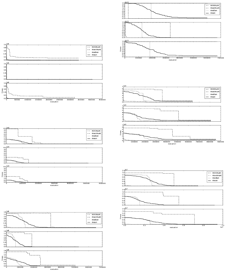
Figure 2: top: C
o
, middle: A
f act
, bottom: C
l
Fitness
progress when approximating f
1
from tab. 4. The evolu-
tionary process is started on f
1
.
Figure 3: top: C
o
, middle: A
f act
, bottom: C
l
Fitness
progress when approximating f
2
from tab. 4. The environ-
ment is switched from f
1
to f
2
without restarting.
Figure 4: top: C
o
, middle: A
f act
, bottom: C
l
Fitness
progress when approximating f
3
from tab. 4. The environ-
ment is switched from f
2
to f
3
without restarting.
A symbolic regression problem has been used to com-
pare performance of the algorithms. The goal of
those algorithms is to evolve a function whose out-
put matches as closely as possible the output that is
Figure 5: top: C
o
, middle: A
f act
, bottom: C
l
Fitness
progress when approximating f
4
from tab. 4. The environ-
ment is switched from f
3
to f
4
without restarting.
Figure 6: top: C
o
, middle: A
f act
, bottom: C
l
Fitness
progress when approximating f
5
from tab. 4. The environ-
ment is switched from f
4
to f
5
without restarting.
Figure 7: top: C
o
, middle: A
f act
, bottom: C
l
Fitness
progress when approximating f
6
from tab. 4. The environ-
ment is switched from f
5
to f
6
without restarting.
provided by the training set of n samples. The fitness
value expresses the sum of absolute differences be-
tween the outputs of the evolved function f
e
and the
corresponding expected outputs y for all input values
x. The goal is to minimise the computed fitness value
(1).
f it
val
=
n
∑
i=1
|
y
i
− f
e
(x
i
)
|
(1)
The experiments have been divided into several
classes. Most of the algorithm settings are shared be-
Cartesian Genetic Programming in a Changing Environment
207

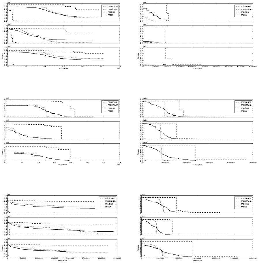
Figure 8: top: C
o
, middle: A
f act
, bottom: C
l
Fitness
progress when approximating f
7
from tab. 4. The environ-
ment is switched from f
6
to f
7
without restarting.
Figure 9: top: C
o
, middle: A
f act
, bottom: C
l
Fitness
progress when approximating f
8
from tab. 4. The environ-
ment is switched from f
7
to f
8
without restarting.
Figure 10: top: C
o
, middle: A
f act
, bottom: C
l
Fitness
progress when approximating f
7
from tab. 5. The evolu-
tionary process is started on f
7
.
tween the experiments in order to be able to compare
the performance of the (1 + λ) evolutionary strategy
and the ALPS CGP algorithm variant. The genome
parameters are summarised in tab. 2. The genome lay-
out has been chosen so it can provide maximal degree
of variability.
Parameters related to genome configuration do not
change and are common for all experiments. The task
is to compare the algorithms by the means of the abi-
lity to maintain convergence and also by the means
of speed. Because population sizes of the algorithms
Figure 11: top: C
o
, middle: A
f act
, bottom: C
l
Fitness
progress when approximating f
71
from tab. 5. The envi-
ronment is switched from f
7
to f
71
without restarting.
Figure 12: top: C
o
, middle: A
f act
, bottom: C
l
Fitness
progress when approximating f
72
from tab. 5. The envi-
ronment is switched from f
71
to f
72
without restarting.
Figure 13: top: C
o
, middle: A
f act
, bottom: C
l
Fitness
progress when approximating f
73
from tab. 5. The envi-
ronment is switched from f
72
to f
73
without restarting.
differ then the progress of the evolutionary process is
not measured in generations. The number of fitness
function invocation is being used instead. This gives
a more precise information about the actual algorithm
performance.
The set of primitive functions Γ contains binary
functions listed in tab. 3. The secure division opera-
tion returns 1 if the divisor is equal to 0.
The set of primitive function has been extended
with a set of constants which act as constant functions
with arbitrary arity. The used constants are: 0, 0.0001,
ECTA 2015 - 7th International Conference on Evolutionary Computation Theory and Applications
208

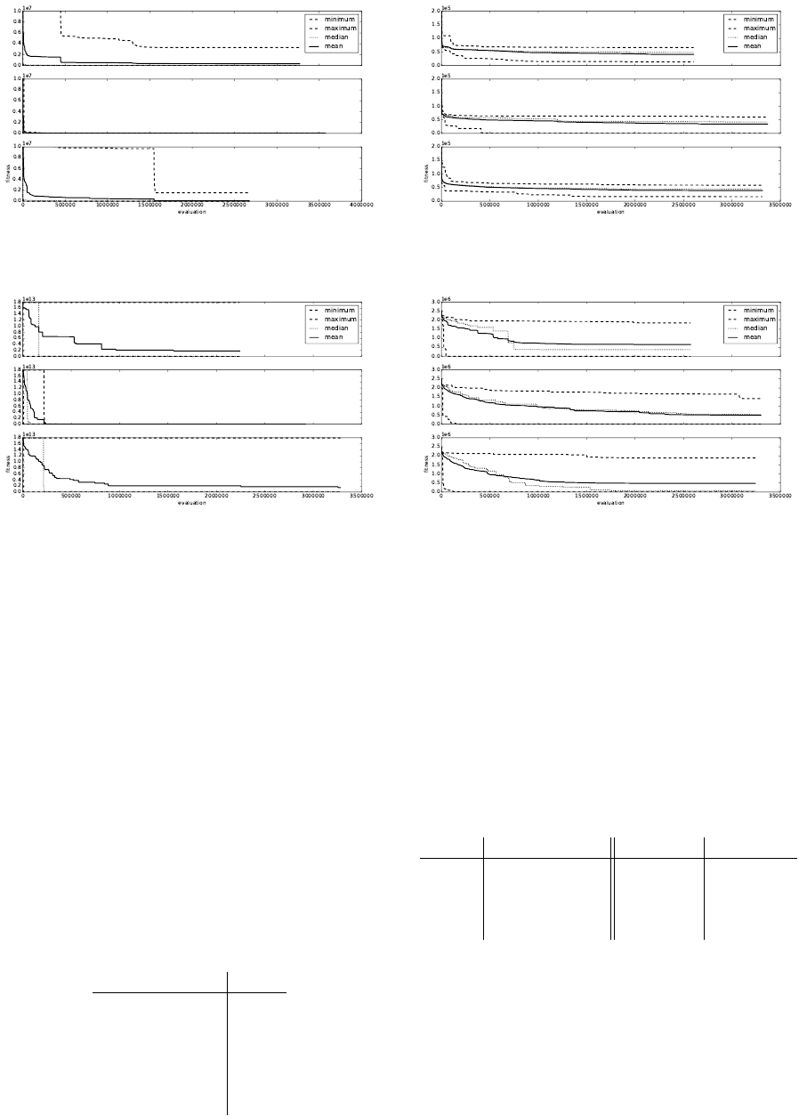
Figure 14: top: C
o
, middle: A
f act
, bottom: C
l
Fitness
progress when approximating f
3
from tab. 4. The evolu-
tionary process is started directly on f
3
.
Figure 15: top: C
o
, middle: A
f act
, bottom: C
l
Fitness
progress when approximating f
4
from tab. 4. The evolu-
tionary process is started directly on f
4
.
0.0002, 0.0005, 0.001, 0.002, 0.005, 0.01, 0.02, 0.05,
0.1, 0.2, 0.5, 1, 2, 5, 10, 20, 50, 100, 200 and 500.
These constant functions ignore any of their inputs
and always return their respective value. That makes
them interchangeable with any of the remaining bi-
nary functions in the function set Γ.
All experiments use a software implementation of
CGP. The algorithm was implemented using the C
programming language in order to achieve reasonable
performance. Some code optimisations have been
used, e.g. avoiding dynamic memory allocations. A
technique of achieving additional performance gain in
CPU-based CGP implementations has been published
(Va
ˇ
s
´
ı
ˇ
cek and Slan
´
y, 2012), however, it has not been
applied in this implementation.
Table 2: Parameters related to the CGP genome as they have
been used in the experiments.
name value
inputs n
i
1
outputs n
o
1
rows n
r
1
columns n
c
100
level-back l 100
mutation rate µ
r
3%
Figure 16: top: C
o
, middle: A
f act
, bottom: C
l
Fitness
progress when approximating f
5
from tab. 4. The evolu-
tionary process is started directly on f
5
.
Figure 17: top: C
o
, middle: A
f act
, bottom: C
l
Fitness
progress when approximating f
7
from tab. 4. The evolu-
tionary process is started directly on f
7
.
The experiments have been performed on a Linux
system containing a X5650 Xeon CPU. The pro-
gramme was started using a starting training set. A
signal has been issued in regular 5-minute intervals
causing the programme to load a subsequent training
set thus causing a sudden change in the environment.
Memory usage has been of little concern as it is in this
case bounded by the training set size and the number
of evaluated phenotype nodes.
Table 3: Functions used as building components. These
functions operate on 32-bit floating point numbers.
func. descr. func. descr.
a + b addition max(a,b) maximum
a − b subtraction min(a,b) minimum
a · b multiplication (a + b)/2 average
a ÷
s
b secure division
Only active nodes are used when evaluating the
fitness, that is the main reason why the application
manages to perform different numbers of evaluations
during the intervals.
3.1 Changing Environment I
In this set of experiments three algorithms have been
Cartesian Genetic Programming in a Changing Environment
209

investigated:
C
o
denotes the ordinary (1 + λ) evolutionary strategy
where λ = 7.
A
f act
denotes the ALPS CGP algorithm variant with a
factorial ageing scheme. The population consists of 5
layers with 8 individuals each. The age-gap parame-
ter is set to 20. The bottom layer is randomised every
200 generations.
C
l
denotes a (1 + λ) strategy algorithm that uses a
large population. The size of the population has been
increased to the size of 40 individuals in order to
match the maximal size of the A
f act
algorithm.
The functions that have been used to generate the
training sets are listed in tab. 4. These polynomials
have been chosen at random. The training sets have
been used throughout the experiments in the order as
they are listed. The training sets consist of equidistant
floating point samples that have been obtained on the
interval ranging from −10.0 to 10.0 with the step of
0.01.
The aim of this experiment is to evaluate how
the algorithms behave in a changing environment –
i.e. how the algorithms cope with sudden changes in
the environments. The environment is changed after
every 5 minutes. The evolutionary algorithms retain
their population structure when the changes occur.
The observed behaviour is summarised in figures 2,
3, 4, 5, 6, 6, 7, 8 and 9. Changes in the environment
occur at evaluation 0 in every mentioned figure except
fig. 2 when the evolution is started.
The figures show the progress of the best achieved
fitness value of 60 experimental runs. The values on
the x-axis are re-sampled so that the number of eva-
luation starts from 0 for every function although the
evolution process does not stop as the environment
changes from f
n
to f
n+1
. Because the total number
of evaluation during the fixed time interval varies it
could be difficult to read the graphs (especially when
comparing the data) with different x-bases.
Four lines are depicted in these graphs. At each
Table 4: Functions used in the changing environment exper-
iments.
function expression
f
1
x
4
+ x
3
+ x
2
+ x
f
2
3x
3
+ 2x
2
+ 3x + 1
f
3
4x
5
− 3x − 20x + 197
f
4
(2x
3
+ 7x
2
− 19x − 11)/(x
4
− 3x
3
+ 2)
f
5
(2x
5
− 4x
3
+ 2x)/(2x
2
+ x − 14)
f
6
3x
4
− 8x
3
+ 2x
f
7
(5x
4
− x
2
+ 2x)/(x
2
+ 7x + 5)
f
8
2x
4
− 10x
2
+ 2x
step in the evolution they display the best, worst and
average achieved best fitness values out of 60 experi-
mental runs. Additionally, the median of all achieved
fitness values is displayed. This gives a hint where the
boundary between the better and the worse half of all
experimental runs is.
3.2 Changing Environment II
In this set of experiments less abrupt changes in the
environment have been simulated. The polynomial
f
7
has been used. The expression has been randomly
modified in each step. Expressions that are the being
approximated are listed in tab. 5.
Figures 10, 11, 12, 13 illustrate the observed be-
haviour. Changes in the environment occur at evalua-
tion 0 in every mentioned figure except fig. 10 when
the evolution is started. Except for the approximated
data the experimental set-up matches the setting listed
in sec. 3.1.
Theoretically, parts of the already evolved
genomes could be reused when an environment
change occurs. Judging from the observed behaviour
this could have happened in fig. 11.
3.3 Static Environment
This set of experiments has been performed on same
data as in sec. 3.1. The goal was to find out whether
there is a difference between the case in which the
algorithm is freshly started or when the algorithm has
to adapt an already present population.
Experimental set-up again matches the settings
from sec. 3.1. The algorithms are restarted every time
a change in the environment occurs. Again all experi-
ments are run for 5 minutes and are repeated 60 times.
Observer behaviour is illustrated in figures 14, 15, 16
and 17.
All of the algorithms show faster convergence
rates when compared with figures from sec. 3.1. In the
first set of experiments the environments have been
changed without restarting the evolutionary process.
At the point of environment change the population is
already flooded with alleles that have evolved in the
old environment and which are rendered useless by
Table 5: Functions used in the changing environment exper-
iments.
function expression
f
7
(5x
4
− x
2
+ 2x)/(x
2
+ 7x + 5)
f
71
(5x
4
− x
2
+ 2x)/(x
2
· 7x + 5)
f
72
(5x
4
− x
10
+ 2x)/(x
2
− 7x + 5)
f
73
(5x
4
− x
10
+ 2x)/x
2
− 7x + 5
ECTA 2015 - 7th International Conference on Evolutionary Computation Theory and Applications
210

the changed environment. In the set of experiments
described in this section the process always starts with
completely randomly initialised population.
3.4 Summary
Nearly all figures show that the ALPS CGP algorithm
behaves best by the means of the worst case scenario
and by the means of average achieved values. The
ALPS variant has also been able to find better solution
more quickly. It has also been able to find solutions
with better fitness in cases where no perfect solution
could be found.
4 CONCLUSIONS
The experiments show that the ALPS CGP algorithm
exerts better adaptation than the ordinary CGP algo-
rithm regardless of the population size. In most cases
the ALPS variant exhibits the best behaviour in the
worst case scenarios. When comparing the average
behaviour, then again it shows the best progress most
of the time. Moreover, in cases when no optimal
solution could be found the ALPS variant was able
to achieve better solutions than the remaining algo-
rithms. Age tags are added and additional comparison
of the tags is required in order to maintain the popu-
lation structure. One could argue that it increases the
memory consumption because of the increased pop-
ulation size. Usually, the memory required for stor-
ing the training set surpasses the memory needed for
holding the genotypes. Whenever abrupt changes in
the environment are going to happen then it is better
to restart the evolution from scratch rather than go-
ing on with adaptation to the changes. It would be
interesting to quantify the amount of changes to the
environment where it would be better to keep the evo-
lution running.
ACKNOWLEDGEMENTS
This work was supported by Brno University of Tech-
nology project FIT-S-14-2297.
REFERENCES
Collins, M. (2006). Finding needles in haystacks is harder
with neutrality. Genetic Programming and Evolvable
Machines, 7(2):131–144.
Ebner, M., Shackleton, M., and Shipman, R. (2001). How
neutral networks influence evolvability. Complexity,
7(2):19–33.
Harding, S. L. (2008). Evolution of image filters on graph-
ics processor units using cartesian genetic program-
ming. In IEEE Congress on Evolutionary Computa-
tion, pages 1921–1928. IEEE.
Hornby, G. S. (2006). ALPS: the age-layered population
structure for reducing the problem of premature con-
vergence. In GECCO ’06: Proceedings of the 8th an-
nual conference on Genetic and evolutionary compu-
tation, pages 815–822, New York, NY, USA. ACM.
Koza, J. R. (1992). Genetic Programming: On the Pro-
gramming of Computers by Means of Natural Selec-
tion. MIT Press, Cambridge.
Miller, J. F. (1999). An empirical study of the efficiency
of learning boolean functions using a cartesian ge-
netic programming approach. In Proceedings of the
Genetic and Evolutionary Computation Conference,
volume 2, pages 1135–1142, Orlando, Florida, USA.
Morgan Kaufmann.
Miller, J. F. and Smith, S. L. (2006). Redundancy and com-
putational efficiency in cartesian genetic program-
ming. IEEE Transactions on Evolutionary Computa-
tion, 10(2):167–174.
Miller, J. F. and Thomson, P. (2000). Cartesian genetic pro-
gramming. In Proceedings of the 3rd European Con-
ference on Genetic Programming, volume 1802, pages
121–132. Springer.
Slan
´
y, K. (2009). Comparison of CGP and age-layered
CGP performance in image operator evolution. In Ge-
netic Programming, 12th European Conference, Eu-
roGP 2009, volume 2009 of Lecture Notes in Com-
puter Science, 5481, pages 351–361. Springer Verlag.
Va
ˇ
s
´
ı
ˇ
cek, Z. and Sekanina, L. (2007). Evaluation of a new
platform for image filter evolution. In Proc. of the
2007 NASA/ESA Conference on Adaptive Hardware
and Systems, pages 577–584. IEEE Computer Society.
Va
ˇ
s
´
ı
ˇ
cek, Z. and Slan
´
y, K. (2012). Efficient phenotype eva-
luation in cartesian genetic programming. In Proceed-
ings of the 15th European Conference on Genetic Pro-
gramming, LNCS 7244, pages 266–278. Springer Ver-
lag.
Walker, J. A. and Miller, J. F. (2005). Investigating the per-
formance of module acquisition in cartesian genetic
programming. In GECCO ’05: Proceedings of the
2005 conference on Genetic and evolutionary compu-
tation, pages 1649–1656, New York, NY, USA. ACM.
Yu, T. and Miller, J. F. (2001). Neutrality and the evolv-
ability of boolean function landscape. In EuroGP
’01: Proceedings of the 4th European Conference on
Genetic Programming, pages 204–217, London, UK.
Springer-Verlag.
Cartesian Genetic Programming in a Changing Environment
211