A Yet Faster Version of Complex-valued Multilayer Perceptron Learning

using Singular Regions and Search Pruning

Seiya Satoh and Ryohei Nakano

Department of Computer Science, Chubu University, 1200 Matsumoto-cho, Kasugai 487-8501, Japan

Keywords:

Complex-valued Multilayer Perceptron, Learning Method, Singular Region, Search Pruning.

Abstract:

In the search space of a complex-valued multilayer perceptron having J hidden units, C-MLP(J), there are

singular regions, where the gradient is zero. Although singular regions cause serious stagnation of learning,

there exist narrow descending paths from the regions. Based on this observation, a completely new learning

method called C-SSF (complex singularity stairs following) 1.0 was proposed, which utilizes singular regions

to generate starting points of C-MLP(J) search. Although C-SSF1.0 ﬁnds excellent solutions of successive

C-MLPs, it takes long CPU time because the number of searches increases as J gets larger. To deal with this

problem, C-SSF1.1 was proposed, a few times faster by the introduction of search pruning, but it still remained

unsatisfactory. In this paper we propose a yet faster C-SSF1.3, going further with search pruning, and then

evaluate the method in terms of solution quality and processing time.

1 INTRODUCTION

Complex-valued neural networks (Hirose, 2012) have

the attractive features real-valued ones don’t have. A

complex-valued multilayer perceptron (C-MLP) can

naturally represent a periodic and/or unbounded func-

tion, which is not easy at all for a real-valued MLP.

Among learning methods of C-MLPs, complex

back propagation (C-BP) (Kim and Guest, 1990; Le-

ung and Haykin, 1991) is basic and well-known.

A higher-order learning method was proposed to

get better performance (Amin et al., 2011). Com-

plex Broyden-Fletcher-Goldfarb-Shanno (C-BFGS)

(Suzumura and Nakano, 2013) ﬁnds nice solutions af-

ter many independent runs.

There exist ﬂat subspaces called singular regions

in the C-MLP search space (Nitta, 2013), as is the

case with a real-valued MLP (Fukumizu and Amari,

2000). Singular regions have been avoided (Amari,

1998) because they cause serious stagnation of learn-

ing. However, they can be utilized as excellent initial

points when we perform search for successive num-

bers of hidden units. This viewpoint led to the in-

vention of a completely new learning method. Ac-

tually, a method called SSF (Singularity Stairs Fol-

lowing) (Satoh and Nakano, 2013) was proposed

for real-valued MLPs, utilizing reducibility mapping

(Fukumizu and Amari, 2000) and eigenvector descent

(Satoh and Nakano, 2012). It stably and successively

found excellent solutions.

Recently a complex version of SSF, called C-SSF

1.0, was proposed (Satoh and Nakano, 2014), uti-

lizing complex reducibility mapping (Nitta, 2004),

eigenvector descent, and C-BFGS. It stably found ex-

cellent solutions in C-MLP search space, whose so-

lution quality was better than C-BFGS. However, it

took several times longer than C-BFGS. To make C-

SSF1.0 faster, C-SSF1.1 (Satoh and Nakano, 2015)

was proposed by introducing search pruning. It ran a

few times faster than C-SSF1.0 without losing the su-

perb solution quality, but still remained unsatisfactory

in processing time.

This paper proposes a yet faster version of C-SSF

called C-SSF1.3 by introducing two contrivances:

putting a ceiling on the number of searches and utiliz-

ing multiple best solutions to generate starting points.

Our experiments compare solution quality and pro-

cessing time of the proposed C-SSF1.3 with those of

C-SSF1.1, C-BP, and C-BFGS.

2 SINGULAR REGIONS

This section explains how singular regions are gener-

ated. Consider a complex-valued MLP with J hidden

units, C-MLP(J), whose output is f

122

Satoh, S. and Nakano, R..

A Yet Faster Version of Complex-valued Multilayer Perceptron Learning using Singular Regions and Search Pruning.

In Proceedings of the 7th International Joint Conference on Computational Intelligence (IJCCI 2015) - Volume 3: NCTA, pages 122-129

ISBN: 978-989-758-157-1

(x;θ

) = w

∑

j=1

, z

≡ g(w

x) (1)

Here θ

= {w

, j = 1,··· , J} is a parameter

vector. Input x, weights w

, w

, output f

, and teacher

signal y are all complex. Given data {(x

),µ =

1,··· ,N}, we want to ﬁnd θ

minimizing the follow-

ing.

∑

µ=1

, δ

≡ f

;θ

) − y

(2)

Next, consider C-MLP(J−1) with J−1 hidden units.

Its output is f

J−1

(x;θ

J−1

) = u

J−1

∑

j=1

, v

≡ g(u

x) (3)

Here θ

J−1

= {u

, j = 1,··· ,J − 1} is a param-

eter vector of C-MLP(J−1), and let the optimal θ

J−1

Sussmann (Sussmann, 1992) pointed out the

uniqueness and reducibility of real-valued MLPs.

Much the same uniqueness and reducibility hold for

complex-valued MLPs (Nitta, 2004). Now consider

three reducibility mappings α, β, and γ; then, apply

α, β, and γ to the optimal

J−1

to get

, and

respectively.

J−1

−→

J−1

−→

J−1

−→

≡ {θ

= bu

, w

=0,

= bu

j−1

=bu

j−1

, j=2,··· ,J} (4)

≡ {θ

g(w

)= bu

=[w

,0,··· ,0]

= bu

j−1

= bu

j−1

, j=2,··· ,J} (5)

≡ {θ

= bu

m−1

=bu

m−1

= bu

j−1

=bu

j−1

, j∈{2,··· ,J}\{m}} (6)

Now, we have the following singular regions.

(1) The intersection of

and

forms singular re-

gion

αβ

, where only w

is free. In the singular re-

gion the following hold:

= bu

, w

= 0, w

= [w

,0,··· ,0]

= bu

j−1

, w

= bu

j−1

, j = 2,··· ,J.

(2)

is a singular region, where the following

holds: w

+ w

= bu

m−1

, m=2, · · · ,J.

After ﬁnishing learning of C-MLP(J−1), C-SSF

starts learning of C-MLP(J) from points in the sin-

gular region of C-MLP(J). Since the gradient is zero

all over the singular region, the gradient won’t give

us any information in which direction to go. Thus

we employ eigenvector descent (Satoh and Nakano,

2012). Picking up a negative eigenvalue, we have two

search directions based on its eigenvector.

3 C-SSF

This section describes the former versions and the

proposed version of C-SSF (Complex Singularity

Stairs Following). C-SSF learns C-MLPs.

3.1 Basic Framework

The origin of C-SSF is C-SSF1.0 (Satoh and Nakano,

2014). C-SSF starts search from C-MLP(J=1) and

then gradually increases the number of hidden units J

one by one until J

max

. When searching C-MLP(J), the

method applies reducibility mapping to the optimum

of C-MLP(J−1) to get two kinds of singular regions

αβ

and

. When starting search from the singu-

lar region, the method employs eigenvector descent

(Satoh and Nakano, 2012), which ﬁnds descending

directions, and from then on employs complex BFGS

(C-BFGS). The general ﬂow of C-SSF1.0 is given be-

low. Let {w

(J)

, j = 1,··· , J} denote param-

eters of C-MLP(J).

Here we give notes on the implementation used

in our experiments. In Algorithm 1, p in steps 1.1

and 2.1.1 is free and was set to −1, 0, and 1. More-

over, q in step 2.2.1 is also free and was set to 0.5,

1.0, and 1.5, which correspond to internal division,

boundary, and external division respectively. In Algo-

rithm 2, the golden section search (Luenberger, 1984)

was employed as a line search to ﬁnd the suitable step

length.

C-SSF has the following characteristics (Satoh

and Nakano, 2014; Satoh and Nakano, 2015).

(1) The excellent solution of C-MLP(J) will be ob-

tained one after another for J=1,···,J

max

. C-SSF guar-

antees that training error of C-MLP(J) is smaller than

that of C-MLP(J−1) since C-SSF descends in C-

MLP(J) search space from the singular regions cor-

responding to the optimum of C-MLP(J−1). This

monotonic feature will be quite useful for model se-

lection. However, such monotonic decrease of train-

ing error is not guaranteed for existing methods.

(2) C-SSF runs without using random number, mean-

ing it always ﬁnds the same set of solutions.

A Yet Faster Version of Complex-valued Multilayer Perceptron Learning using Singular Regions and Search Pruning

123

Algorithm 1: C-SSF Method (ver 1.0 or 1.1).

step 1. Search for MLP(1)

1.1 Set an initial point on

αβ

(1)

←

y, w

(1)

← 0, w

(1)

← [p,0,··· ,0]

1.2 Search

from singular region

1.3 Store the best as bw

(1)

, bw

(1)

, bw

(1)

; J ← 2.

step 2. Search for MLP(J)

while J ≤ J

max

2.1 Search from

αβ

2.1.1 Set

an initial point on

αβ

2.1.2 Search

from singular region

2.2 Search from

for m = 2,··· , J do

2.2.1 Set an initial point on

2.2.2 Search

from singular region

end for

2.3 Get the best among all solutions obtained

in steps 2.1 and 2.2, and store it as bw

(J)

, bw

(J)

, j = 1,··· ,J. Then, J ← J + 1.

end while

Algorithm 2: Search from singular region.

step 1. Calculate the Hessian and get all the nega-

tive eigenvalues and their eigenvectors.

step 2.

for each negative eigenvalue with its eigenvector u

2.1 Perform a line search in the direction of u,

start search using C-BFGS afterward, and keep

the solution.

2.2 Perform a line search in the direction of −u,

start search using C-BFGS afterward, and keep

the solution.

end for

3.2 Search Pruning

C-SSF1.0 stably found excellent solutions, better than

C-BFGS. However, it took several times longer than

C-BFGS because the number of searches got larger

and larger as the number of hidden units J increased.

Thus, a faster version C-SSF1.1 (Satoh and Nakano,

2015) was proposed by introducing search pruning.

The general ﬂow of C-SSF1.1 is the same as Al-

gorithm 1 since search pruning is embedded in search

using C-BFGS at steps 2.1 and 2.2 of Algorithm

2. Although search pruning is explained in detail in

(Satoh and Nakano, 2015), the main point is shown

below.

Algorithm 3: Set an initial point on

αβ

(J)

← bw

(J−1)

(J)

←0, w

(J)

←[p, 0,··· ,0]

(J)

← bw

(J−1)

j−1

, w

(J)

← bw

(J−1)

j−1

, j=2,··· , J

Algorithm 4: Set an initial point on

(J)

← bw

(J−1)

(J)

← q × bw

(J−1)

m−1

, w

(J)

← bw

(J−1)

m−1

(J)

← (1 − q) × bw

(J−1)

m−1

, w

(J)

← bw

(J−1)

m−1

(J)

← bw

(J−1)

j−1

, w

(J)

← bw

(J−1)

j−1

j ∈ {2, · · · ,J} \ {m}

Let θ

(t)

and φ

(τ)

be a current search point and

a point stored during a previous search respectively.

Since d = (··· ,d

,···)

is a normalizing vector, v

(t)

and r

(τ)

are normalized points. The normalization is

introduced to prevent any weight having a large abso-

lute value from inﬂuencing the decision too much.

←









(t−1)



(1 < |θ

(t−1)

(|θ

(t−1)

| ≤ 1)

(7)

(t)

← diag(d) θ

(t)

(8)

(t−1)

← diag(d) θ

(t−1)

(9)

(τ)

← diag(d) φ

(τ)

, τ = 1,··· , T (10)

Here m = 1,··· ,2M, where M is the number of com-

plex weights. Let T be the number of points stored so

far, and diag(d) is a diagonal matrix whose diagonal

elements are d.

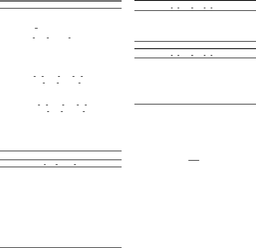
See Figure 1. Now consider a line L

through two

points r

(τ−1)

and r

(τ)

, and a line L

through two points

(t−1)

and v

(t)

. Then consider a line L

perpendicular

to each of L

and L

. Note that line L

includes the

shortest line segment ℓ between L

and L

. Based on

this ℓ, we decide whether the current search route is to

merge onto a previous search route. We can calculate

ℓ, which can be represented as below.

ℓ = (r

(τ−1)

+ a

∆r

(τ)

) − (v

(t−1)

+ a

∆v

(t)

) (11)

∆r

(τ)

≡ r

(τ)

− r

(τ−1)

, ∆v

(t)

≡ v

(t)

− v

(t−1)

By solving min

ℓ

ℓ, unknown a

and a

can be de-

termined. The following are the condition for ℓ to

start from a point between v

(t−1)

and v

(t)

and to end at

a point between r

(τ−1)

and r

(τ)

0 ≤ a

≤ 1, 0 ≤ a

≤ 1 (12)

If ℓ does not satisfy the condition eq.(12) for any τ =

1,··· ,T, we consider the current search route does

NCTA 2015 - 7th International Conference on Neural Computation Theory and Applications

124

(τ)

(t)

(τ−1)

(t−1)

(t−2)

(τ−2)

(τ−3)

(τ−4)

Figure 1: Conceptual Diagram of Search Pruning of C-

SSF1.1.

not merge onto any previous route. If the condition

holds for a certain τ, however, we check whether the

current search is to be pruned. The current search is

pruned if the absolute value of each element of ℓ is

smaller than predeﬁned ε.

Here implementation details in our experiments

are described. Checking of search pruning and stor-

ing of current points are carried out at intervals of 100

search steps. Moreover, we set ε = 0.3 for a threshold

of search route proximity.

3.3 Proposed Method: C-SSF1.3

C-SSF1.1 ran a few times faster than C-SSF1.0 with-

out losing the excellent solution quality, but still re-

mained unsatisfactory in processing time for a larger

model. C-SSF1.1 needed to be made even faster; thus,

this paper proposes a yet faster version C-SSF1.3.

Since the key point is to decrease the number of

searches, we decided to put a ceiling S

max

on the

number; however, we should not lose excellent so-

lutions by doing so. All of the limited number S

max

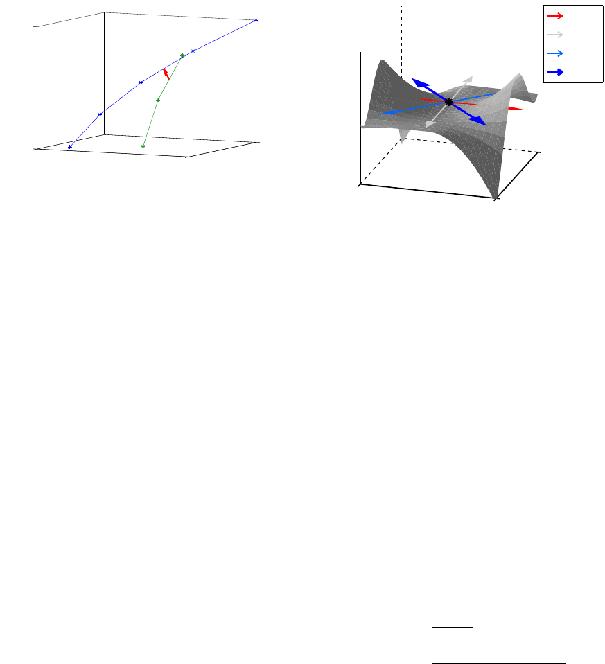
of searches should start in the promising directions.

Note that the decision whether or not this direction

will lead to an excellent solution should be made at a

starting point. We assumed the larger convex curva-

ture at a starting point, the better solution at the end

of the search. See Figure 2.

To implement this, we calculate eigenvalues of

all initial points on the singular regions

αβ

and

Then, we pick up the limited number of eigenvalues

in ascending order, and perform search using their

eigenvectors.

One more contrivance was introduced into C-

SSF1.3. When C-SSF starts search at one step larger

C-MLP(J), only the best solution of C-MLP(J−1) is

used to create the singular regions. Recently we found

that the best solution of C-MLP(J−1) does not always

lead to the best solution of C-MLP(J) especially for a

very small J. Therefore, we utilize the best R solu-

tions of C-MLP(J−1) to create the singular regions

(>0)

(=0)

(>λ

)

(<λ

)

Figure 2: Conceptual diagram of eigenvectors at a point in

a singular region.

of C-MLP(J) when J ≤ J

. Note that when J ≤ J

the ceiling on the number of searches is not put. The

increase of processing load due to additional searches

will be trivial because J is very small.

In the following experiments, C-SSF1.3 system

parameters were set as S

max

= 100, J

= 3, and R =

4 EXPERIMENTS

The proposed C-SSF1.3 was evaluated using two arti-

ﬁcial data sets. That is, the performance of C-SSF1.3

was compared with former version C-SSF1.1, batch-

type complex BP with line search (C-BP), and com-

plex BFGS (C-BFGS).

In a C-MLP an activation function plays an impor-

tant role. We employed the following σ(z) (Kim and

Guest, 1990; Leung and Haykin, 1991) for a hidden

unit. When z is a complex number (z = a+ i b), σ(z)

is periodic and unbounded.

σ(z) =

1+ e

−z

1+ e

−a

cosb+ ie

−a

sinb

1+ 2e

−a

cosb+ e

−2a

(13)

Real and imaginary parts of initial weights for C-

BP and C-BFGS were randomly selected from the

range (−1,1). For each J, C-BP or C-BFGS was per-

formed 100 times changing initial weights.

Each run of any learning method was terminated

when the number of sweeps exceeded 10,000 or the

step length got smaller than 10

−16

A Yet Faster Version of Complex-valued Multilayer Perceptron Learning using Singular Regions and Search Pruning

125

4.1 Experiments using Artiﬁcial Data 1

Artiﬁcial data 1 was generated using a C-MLP hav-

ing the following weights with J = 4. A PC with In-

tel(R) Xeon(R) E5-2687W 3.10GHz and 32GB mem-

ory was used together with MATLAB2014a.

)

= (−3+ 1i,−1+ 1i,1+ 1i,0+ 5i,5− 4i),

)







−2+ 3i 0− 5i −4− 5i −1+ 1i

4+ 0i −2+ 2i −1+ 2i −2+ 2i

−3+ 1i 0− 2i −4− 4i 4+ 1i

4+ 4i 1+ 4i 3+ 0i −4− 1i

0− 5i 5+ 3i −1− 5i 3− 1i

−5− 2i −4+ 2i 3− 5i 5+ 4i







(14)

The real and imaginary parts of input x

were ran-

domly selected from the range (0,1). Teacher sig-

nal y

was generated by adding small Gaussian noise

N (0,0.01

) to both real and imaginary parts of the

output. The size of training data was 500 (N = 500),

and the maximum number of hidden units was set to

6 (J

max

= 6). Test data of 1,000 data points without

noise was generated independently of training data.

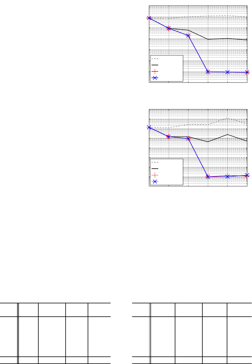
Figures 3 (a) and (b) show minimum training er-

ror and the corresponding test error respectively. C-

BP could not decrease training error and showed very

poor generalization. C-BFGS basically decreased

training error as J got larger; however, its test error

showed the slight up-and-down movement. Both fast

versions of C-SSF showed much the same results for

training and test, much better than those of C-BFGS

for J ≥ 4. Note also that C-SSF monotonically de-

creased training error. Both versions of C-SSF and

C-BFGS minimized test error at J = 4, which is cor-

rect.

Table 1 shows the number of searches for artiﬁ-

cial data 1. The numbers of each C-SSF include the

ones of pruned searches. Note that the numbers of

each C-SSF for J = 2 or 3 were larger than 100 be-

cause multiple best solutions were utilized to create

starting points. The total number of C-SSF1.3 was 29

% (0.71=791/1108) smaller than that of C-SSF1.1.

Table 1: Numbers of searches for artiﬁcial data 1.

J C-BP C-BFGS C-SSF C-SSF

1.1 1.3

1 100 100 38 38

100 100 132 132

3 100 100 321 321

100 100 160 100

5 100 100 220 100

100 100 237 100

total 600 600 1108 791

1 2 3 4 5 6

−2

−1

Training error

C−BP

C−BFGS

C−SSF1.1

C−SSF1.3

(a) Training error.

1 2 3 4 5 6

−2

−1

Test error

C−BP

C−BFGS

C−SSF1.1

C−SSF1.3

(b) Test error.

Figure 3: Training and test errors for artiﬁcial data 1.

Table 2 shows CPU time required by each method

for artiﬁcial data 1. C-BP spent the longest time 443

minutes in total, which may mean it easily got stuck in

poor local minima, and could not escape from them.

C-SSF1.3 was 1.23 (=742/602) times faster than C-

SSF1.1, and C-BFGS was in the middle of the two.

CPU time required by C-BFGS increased as J got

larger, while CPU time of C-SSF at J = 3 was a bit

large due to using multiple best solutions for creating

starting points.

Table 2: CPU time for artiﬁcial data 1 (hr:min:sec).

J C-BP C-BFGS C-SSF C-SSF

1.1 1.3

1 0:35:38 0:00:30 0:00:13 0:00:13

0:53:57 0:00:53 0:00:39 0:00:39

3 1:10:27 0:01:08 0:03:09 0:03:09

1:39:13 0:02:18 0:01:19 0:01:00

5 1:22:45 0:02:35 0:02:56 0:02:07

1:41:25 0:03:54 0:04:06 0:02:53

total 7:23:24 0:11:19 0:12:22 0:10:02

NCTA 2015 - 7th International Conference on Neural Computation Theory and Applications

126

4.2 Experiments using Artiﬁcial Data 2

Artiﬁcial data 2 was generated using the follow-

ing logarithmic spirals. How ﬂexibly C-MLP can

represent this heavily swirling function was evalu-

ated. XPS 8300 with Intel(R) Core i7-2600 3.40GHz

and 12GB memory was used together with MAT-

LAB2014a.

y = {0.001e

0.1φ

+ 2.5e

−0.1φ

+ 0.1e

0.05φ

}

2iφ

+ e

5i(φ+π/3)

+ e

12iφ

+ e

15iφ

where φ = 2πx (15)

The real part of input x

was randomly selected from

the range (0,10), and the imaginary part was set to

zero. Teacher signal y

was generated by adding small

Gaussian noise N (0, 0.01

) to both real and imag-

inary parts of the output. The size of training data

was 1,000 (N = 1,000), and the maximum number of

hidden units was set to 16 (J

max

= 16). Test data of

1,000 data points without noise was generated from

the range (10,13) of input x, outside of the range of

training.

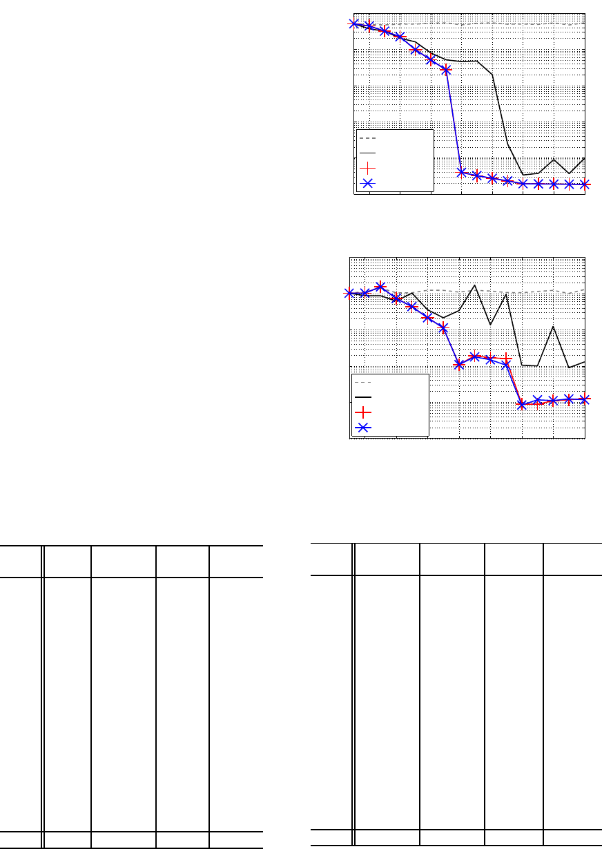
Figures 4 (a) and (b) show minimum training

error and the corresponding test error respectively.

Again C-BP could hardly decrease training error and

showed very poor generalization. C-BFGS basically

decreased training error as J increased, but ﬂuctuated

for J ≥ 12. Both versions of C-SSF showed almost

equivalent results for training and test, monotonically

decreasing training error. Both C-SSF versions indi-

cate J = 12 or 13 may be the best model.

Table 3: Numbers of searches for artiﬁcial data 2.

J C-BP C-BFGS C-SSF C-SSF

1.1 1.3

1 100 100 16 16

2 100 100 81 81

100 100 162 162

4 100 100 70 70

100 100 80 80

6 100 100 177 100

7 100 100 190 100

100 100 269 100

9 100 100 568 100

100 100 306 100

11 100 100 593 100

100 100 583 100

13 100 100 1042 100

100 100 770 100

15 100 100 1664 100

100 100 838 100

total 1600 1600 7409 1509

2 4 6 8 10 12 14 16

−1

Training error

C−BP

C−BFGS

C−SSF1.1

C−SSF1.3

(a) Training error.

2 4 6 8 10 12 14 16

Test error

C−BP

C−BFGS

C−SSF1.1

C−SSF1.3

(b) Test error.

Figure 4: Training and test errors for artiﬁcial data 2.

Table 4: CPU time for artiﬁcial data 2 (hr:min:sec).

J C-BP C-BFGS C-SSF C-SSF

1.1 1.3

1 0:38:58 0:01:03 0:00:10 0:00:10

2 1:11:01 0:01:46 0:02:16 0:02:18

1:12:26 0:03:38 0:05:27 0:05:33

4 1:29:03 0:04:47 0:03:00 0:03:07

1:39:42 0:06:10 0:03:17 0:03:25

6 1:55:47 0:07:22 0:08:27 0:07:08

2:11:15 0:09:22 0:09:16 0:06:26

8 2:22:59 0:11:08 0:14:34 0:07:46

2:33:36 0:13:54 0:22:46 0:06:55

10 2:54:17 0:15:51 0:13:31 0:06:27

3:04:18 0:18:23 0:30:37 0:07:39

12 3:20:16 0:19:35 0:24:39 0:07:27

3:49:26 0:22:03 0:38:24 0:09:32

14 4:00:40 0:26:08 0:24:32 0:06:28

4:12:06 0:25:33 1:04:22 0:06:42

16 4:33:26 0:28:11 0:31:31 0:07:02

total 41:09:15 3:34:55 4:56:48 1:34:04

A Yet Faster Version of Complex-valued Multilayer Perceptron Learning using Singular Regions and Search Pruning

127

−20

Re(y )

Im(y )

Training data

Test data

(a) C-BP(J = 15)

−20

Re(y )

Im(y )

Training data

Test data

(b) C-BFGS(J = 15)

−20

Re(y )

Im(y )

Training data

Test data

−20

Re(y )

Im(y )

Training data

Test data

(d) C-SSF1.3(J = 12)

Figure 5: Outputs of C-MLPs.

Table 3 shows the number of searches of each

method for artiﬁcial data 2. The numbers of each

C-SSF include the ones of pruned searches. The

numbers of each C-SSF for J = 3 were larger than

100 because multiple best solutions were utilized for

J ≤ 3. The total number of C-SSF1.3 was one-ﬁfth

(0.20=1509/7409) of that of C-SSF1.1.

Table 4 shows CPU time required by each method

for artiﬁcial data 2. C-BP spent the longest CPU time

about 41 hours in total. CPU time of C-BFGS grad-

ually increased as J got larger, spending 3.6 hours in

total. C-SSF1.3 was the fastest, 3.2 times (=297/94)

faster than C-SSF1.1, and 2.3 times (=215/94) faster

than C-BFGS. Note that C-SSF1.3 spent about 6 or

7 minutes for each J (≥ 6) except J=13, while C-

SSF1.1 showed a tendency to require more CPU time

as J got larger.

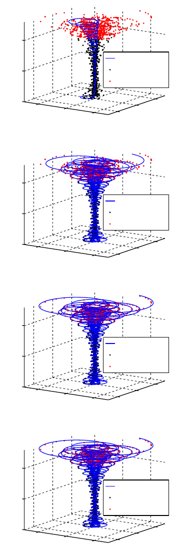
Figures 5 (a), (b), (c) and (d) show the output of

the best models learned by each learning method. The

best model means C-MLP(J) minimizing test error;

J=15 for C-BP and C-BFGS, J=13 for C-SSF1.1, and

J=12 for C-SSF1.3. C-BP could hardly ﬁt the func-

tion for the range (0, 10) and showed very poor gener-

alization for the range (10,13). C-BFGS nicely ﬁtted

the function in the range (0,10), but the amplitude ﬁt-

ting got slightly deviated for the range (10,13). Both

versions of C-SSF very nicely ﬁtted the swirling func-

tion all over the range (0,13) showing excellent gen-

eralization.

5 CONCLUSION

C-SSF is a completely new learning method for a

complex-valued MLP, making good use of singular

regions to stably and successively ﬁnd excellent so-

lutions. We proposed C-SSF1.3 which puts a ceiling

on the search load for larger models and utilizes mul-

tiple best solutions for smaller models. Although the

former versions of C-SSF were rather slow, the pro-

posed C-SSF1.3 ran very fast without losing excellent

solution quality. It ran 3.2 times faster than C-SSF1.1,

2.3 times faster than C-BFGS for a larger problem. In

the future we plan to apply the method to challenging

applications.

ACKNOWLEDGEMENTS

This work was supported by Grants-in-Aid for Sci-

entiﬁc Research (C) 25330294 and Chubu University

Grant 26IS19A.

NCTA 2015 - 7th International Conference on Neural Computation Theory and Applications

128

REFERENCES

S. Amari: Natural gradient works efﬁciently in learning,

Neural Comput., 10(2), 251/276 (1998)

M.F. Amin and et al.: Wirtinger calculus based gradient de-

scent and Levenberg-Marquardt learning algorithms

in complex-valued neural networks, Proc. ICONIP,

550/559 (2011)

K. Fukumizu and S. Amari: Local minima and plateaus in

hierarchical structure of multilayer perceptrons, Neu-

ral Networks, 13(3), 317/327 (2000)

A. Hirose: Complex-Valued Neural Networks, 2nd ed.,

Springer-Verlag, Berlin Heidelberg (2012)

M.S. Kim and C.C. Guest: Modiﬁcation of backpropaga-

tion networks for complex-valued signal processing in

frequency domain, Proc. IJCNN, 3, 27/31 (1990)

H. Leung and S. Haykin: The complex backpropaga-

tion algorithm, IEEE Trans. Signal Process., 39(9),

2101/2104 (1991)

D.G. Luenberger: Linear and nonlinear programming,

Addison-Wesley Publishing Company, Reading, Mas-

sachusetts (1984)

T. Nitta: Reducibility of the complex-valued neural net-

work, Neural Information Processing - Letters and

Reviews, 2(3), 53/56 (2004)

T. Nitta: Local minima in hierarchical structures of

complex-valued neural networks, Neural Networks,

43, 1/7 (2013)

S. Satoh and R. Nakano: Eigen vector descent and line

search for multilayer perceptron, Proc. IAENG Int.

Conf. on AI & Applications (ICAIA’12), 1 1/6 (2012)

S. Satoh and R. Nakano: Fast and stable learning utiliz-

ing singular regions of multilayer perceptron, Neural

Processing Letters, 38(2), 99/115 (2013)

S. Satoh, and R. Nakano: Complex-valued multilayer per-

ceptron search utilizing singular regions of complex-

valued parameter space, Proc. ICANN, 315/322

(2014)

S. Satoh, and R. Nakano: Complex-valued multilayer per-

ceptron learning using singular regions and search

pruning, Proc. IJCNN (to be published) (2015)

H.J. Sussmann: Uniqueness of the weights for minimal

feedforward nets with a given input-output map, Neu-

ral Networks, 5(4), 589/593 (1992)

S. Suzumura and R. Nakano: Complex-valued BFGS

method for complex-valued neural networks, IEICE

Trans. on Information & Systems, J96-D(3), 423/431

(in Japanese) (2013)

A Yet Faster Version of Complex-valued Multilayer Perceptron Learning using Singular Regions and Search Pruning

129