Assessing Vertex Relevance based on Community Detection

Paul Parau, Camelia Lemnaru and Rodica Potolea

Department of Computer Science, Technical University of Cluj-Napoca, Cluj-Napoca, Romania

Keywords:

Vertex Relevance, Commitment, Importance, Relative Commitment, Community Disruption.

Abstract:

The community structure of a network conveys information about the network as a whole, but it can also

provide insightful information about the individual vertices. Identifying the most relevant vertices in a net-

work can prove to be useful, especially in large networks. In this paper, we explore different alternatives for

assessing the relevance of a vertex based on the community structure of the network. We distinguish between

two relevant vertex properties - commitment and importance - and propose a new measure for quantifying

commitment, Relative Commitment. We also propose a strategy for estimating the importance of a vertex,

based on observing the disruption caused by removing it from the network. Ultimately, we propose a vertex

classiﬁcation strategy based on commitment and importance, and discuss the aspects covered by each of the

two properties in capturing the relevance of a vertex.

1 INTRODUCTION

Networks are essential instruments in understanding

many different types of data: social networks (rep-

resenting people and their relationships), biological,

technological or even information networks (New-

man, 2003; Fortunato, 2010). The study of such net-

works becomes harder as the size of the networks in-

creases, and extracting useful information from a net-

work having hundreds of thousands or millions of ver-

tices becomes a real challenge. To extract relevant in-

formation from such networks one must look at their

underlying structural properties. One such property is

their community structure: in networks which have

a community structure, vertices form groups called

communities. The speciﬁc meaning of a community

depends on the data the network is based on. For ex-

ample, in a social network, a community can be a

group of friends, or people who frequently commu-

nicate with each other. Finding the community struc-

ture of a network can help us gain useful insights into

the organization of the network. Applications of com-

munity detection include: making recommendations

to people based on the preferences of other people in

their community, studying the structure of the inter-

net, and analyzing networks of metabolic pathways

or protein interactions (Newman, 2003).

By analyzing the community structure of a net-

work, one can gain very useful macroscopic informa-

tion. But what about the microscopic level? What in-

formation does a community structure convey about

individual vertices? Are some vertices more impor-

tant than others and in what way? Our aim is to ﬁnd

answers to such questions by looking at how vertices

are connected both inside their own community and

outside and how important the vertices and their con-

nections are.

We initially focus on commitment, a property

which quantiﬁes how strongly a vertex belongs to

its community. We analyze two existing mea-

sures for commitment, embeddedness (Lancichinetti

et al., 2010) and signiﬁcance (Rosvall and Bergstrom,

2010), and propose a new measure - Relative Com-

mitment. We show, based on the results of system-

atic experiments, that commitment does not capture

all information pertaining to the relevance of a vertex

and thus we identify another property: importance,

which reveals information about how important a ver-

tex is in its own community. We propose community

disruption as an importance measure which evaluates

the effects of removing that vertex on the community.

Based on commitment and importance, we propose a

categorization of vertices. Our solution can be used

in any type of network. For instance, one can identify

community leaders in a social network or the most

relevant researchers in a scientiﬁc collaboration net-

work.

The rest of the paper is organized as follows: sec-

tion 2 discusses existing research related to measuring

vertex and community structure properties, section 3

Parau, P., Lemnaru, C. and Potolea, R..

Assessing Vertex Relevance based on Community Detection.

In Proceedings of the 7th International Joint Conference on Knowledge Discovery, Knowledge Engineering and Knowledge Management (IC3K 2015) - Volume 1: KDIR, pages 46-56

ISBN: 978-989-758-158-8

describes the datasets and methods used in our exper-

iments, section 4 discusses the results obtained with

existing measures of commitment and in section 5 we

propose a new measure for commitment, describe a

strategy for estimating both vertex and edge impor-

tance and show how vertices can be categorized based

on commitment and importance.

2 RELATED WORK

In this section, after a brief description of commu-

nity detection, we describe existing vertex-level mea-

sures. Additionally, we discuss methods of quantify-

ing higher-level community structure properties, ele-

ments of which we will use throughout this paper.

2.1 Community Detection

A community is commonly deﬁned as an area of the

network where the density of edges inside the com-

munity is greater than the density of the entire net-

work (Newman, 2003; Fortunato, 2010). The ver-

tices in a community usually share some common

traits and/or roles in the network. The collection of

communities in a graph is called community struc-

ture and community detection is the process of ﬁnd-

ing the community structure of a network. Commu-

nities can share vertices (overlapping communities)

and community structures can be hierarchical, with

higher-level communities being composed of lower-

level communities.

There are many approaches for ﬁnding the com-

munity structure of a network. An important cate-

gory of algorithms are hierarchical algorithms, which

build a dendrogram based on a vertex similarity mea-

sure, where each level represents a possible com-

munity structure. The dendrogram can be built in

a top-down (divisive) or bottom-up (agglomerative)

approach (Fortunato and Castellano, 2008). Another

important category, ﬁrst proposed by Newman (New-

man, 2004), are algorithms based on modularity op-

timization, a measure of the quality of the commu-

nity structure in a network. Infomap is a different

type of algorithm proposed by Rosvall and Bergstrom

(Rosvall and Bergstrom, 2008) which works by com-

pressing a description of the probability ﬂow of ran-

dom walks in a network. The algorithm searches

for a community structure which minimizes the de-

scription length of a random walk. Studies evaluating

the performance of community detection algorithms

found the Infomap algorithm to be generally better

performing than alternatives (Lancichinetti and For-

tunato, 2009; Orman et al., 2012).

2.2 Vertex Measures

One of the simplest strategies to quantify the com-

mitment of a vertex to its community is embedded-

ness (Lancichinetti et al., 2010; Orman et al., 2012;

Palla et al., 2007). Embeddedness is a measure that

indicates how many neighbors of a vertex are in the

same community as the vertex and is deﬁned (1) as

the ratio between the internal degree k

(number of

edges inside the community) and the total degree k

of the vertex. For a weighted graph, the formula is

a weighted one, considering the weights of the corre-

sponding edges instead of just counting them.

e =

(1)

As is shown in (Palla et al., 2007), vertices with

low embeddedness have a high likelihood of leaving

the community in the future. In real-world networks,

the majority of the vertices have an embeddedness

e = 1 (Lancichinetti et al., 2010; Orman et al., 2012),

since most of them are located inside their own com-

munities and do not have edges outside. The vertices

that have an embeddedness e < 1 are vertices located

at the fringes of their respective communities.

Also based on degree, Guimera and Amaral

(Guimera and Amaral, 2005) analyze the connectivity

of vertices and propose a number of universal roles for

them. They deﬁne the z-score of a vertex (2), where

is the internal degree of vertex i,

is the average

internal degree of all the vertices in community s

and

is the standard deviation.

−

(2)

Since this measure does not take connections to

vertices in other communities into account, two ver-

tices in the same community, with the same inter-

nal degree but different external degree will have the

same z-score. To distinguish between such vertices,

the authors deﬁne the participation coefﬁcient of a

vertex i as shown in (3), where κ

is the degree with

community s, and k

is the total degree of the vertex.

A vertex with edges exclusively in its own community

has a participation coefﬁcient of 0.

= 1 −

∑

s=1





(3)

Jointly evaluating these measures, the authors de-

ﬁned 7 roles for vertices: based on the value of the

z-score, vertices are community hubs if z

≥ 2.5 and

non-hubs if z

< 2.5. Based on the participation co-

efﬁcient, which indicates how the connections of the

vertex are spread out among the communities of the

Assessing Vertex Relevance based on Community Detection

graph, vertices were further classiﬁed. In increasing

order of participation coefﬁcient, non-hubs were clas-

siﬁed as ultra-peripheral (R1), peripheral (R2), non-

hub connectors (R3) and non-hub kinless (R4) and

hubs were classiﬁed as provincial (R5), connector

(R6) or kinless hubs (R7). In section 5.3, we analyze

the way these universal roles compare to the vertex

categories we propose.

A way to ﬁnd out which vertices are the most sig-

niﬁcant is proposed by Rosvall and Bergstrom (Ros-

vall and Bergstrom, 2010). Their approach, called

signiﬁcance clustering, uses a bootstrap resampling

technique to assess which vertices are signiﬁcant in a

community. The basic idea is to generate a number of

networks derived from the original but with small per-

turbations to their connections and then apply a com-

munity detection algorithm on them. In each com-

munity, the largest subset of vertices that are clus-

tered together in at least 95% of the bootstrap net-

works is found by using simulated annealing. This

subset is called a signiﬁcant subset. Communities are

signiﬁcantly distinct from other communities if their

signiﬁcant subset is not clustered together with any

other signiﬁcant subset in at least 95% of the boot-

strap networks. Since signiﬁcant vertices are unlikely

to leave the community when the network is slightly

perturbed, their signiﬁcance can be considered a mea-

sure of commitment. It is important to note that this

method is independent of the community detection

method used and as such can be used with any algo-

rithm. This approach of generating slightly perturbed

graphs and analyzing differences in community struc-

ture was used in earlier research to determine the sta-

tistical signiﬁcance of the identiﬁed community struc-

ture and will be described in more detail in the follow-

ing section.

2.3 Community Structure Signiﬁcance

In (Karrer et al., 2008), the authors present a method

of measuring the signiﬁcance of a community struc-

ture by determining its robustness to small perturba-

tions. The idea behind this is that a signiﬁcant com-

munity structure will be robust to small perturbations,

whereas a community structure that is not statistically

signiﬁcant will be sensitive to small changes. The

perturbation method they propose modiﬁes the po-

sition of the edges of the network, maintaining the

same number of vertices and edges. Each edge of the

network will be deleted with a probability α. Each

deleted edge will be replaced with a new edge be-

tween two vertices chosen randomly with a proba-

bility given by the expected number of edges. The

expected number of edges between two vertices is de-

ﬁned in equation (4), where k

and k

are the degrees

of the vertices i and j in the original network and m is

the total number of edges.

i j

(4)

Not only does this perturbation method generate

networks with the same number of vertices and edges,

but the expected degree of vertices also remains the

same.

A number of perturbed networks is generated and

the difference between the original community struc-

ture and the community structure of the perturbed net-

works is measured. This is done by calculating an

information theoretic measure called Variation of In-

formation, deﬁned in (5).

V I = −

∑

P(x,y)log

P(x,y)

P(y)

−

∑

P(x,y) log

P(x,y)

P(x)

(5)

Variation of Information measures how different

two community structures are based on the number

of vertices that are clustered together in both struc-

tures. P(x, y) is deﬁned as the number of vertices that

appear in both communities divided by the total num-

ber of vertices, and P(x) and P(y) are deﬁned as the

number of vertices that appear in community X and Y

respectively, divided by the total number of vertices.

This measure can be normalized by 1/log n, where

n is the total number of vertices in the graph. High

Variation of Information between the perturbed com-

munity structures and the original means that the orig-

inal community structure is not statistically signiﬁ-

cant. Similar to signiﬁcance clustering, this method

is independent of the community detection algorithm

used.

Related to the concept of measuring community

structure robustness by perturbing the graph is the re-

search presented in (Albert et al., 2000), which out-

lines a method of assessing the resilience of a network

by measuring its ability to carry information after re-

moving its vertices. The authors found that scale-free

networks are very resilient to random vertex removal

but highly vulnerable to targeted removal of the most

connected vertices.

3 EXPERIMENTAL DATA AND

METHODS

Given that the Infomap algorithm has been found to

be generally better performing than alternatives, we

KDIR 2015 - 7th International Conference on Knowledge Discovery and Information Retrieval

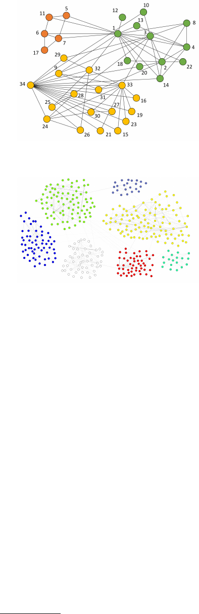
Figure 1: The community structure of the Karate network

as identiﬁed by the Infomap algorithm.

Figure 2: The largest communities in the Netscience net-

work in the top-level community structure, as identiﬁed by

the Infomap algorithm.

have chosen to use this algorithm

in our experiments.

We use two networks in our experiments:

Zachary’s Karate Club (Zachary, 1977) (henceforth

referred to as the Karate network) and a network of

coauthorships in network science compiled by New-

man in (Newman, 2006) (henceforth referred to as

the Netscience network). The Karate network repre-

sented in Figure 1 is one of the ﬁrst and most studied

in network science and is an undirected, unweighted

graph that represents the relationships between mem-

bers of a karate club. It contains 78 edges and 34

vertices which are divided into three communities, as

identiﬁed by the Infomap algorithm. The Netscience

network represented in Figure 2 is an undirected,

weighted graph of scientists working in the ﬁeld of

network theory. It contains 1589 vertices and 2742

edges. The Infomap algorithm found that this network

has a three-level hierarchical community structure.

The results of our experiments indicate that there

are actually two properties of vertices that are relevant

for their relationship with the community: commit-

ment, which quantiﬁes how strongly a vertex belongs

to its community and importance, which should con-

vey information related to the relevance of the vertex

D. Edler and M. Rosvall, The MapEquation software

package, available online at http://www.mapequation.org.

to the structure of its community. Using the Karate

and Netscience networks, we have analyzed measures

that assess both commitment and importance and de-

termined categories of vertices based on these proper-

ties.

4 ANALYSIS OF EXISTING

MEASURES

This section presents an experimental assessment of

existing commitment measures: embeddedness and

signiﬁcance. The evaluations were performed accord-

ing to the methodology described in the previous sec-

tion. We analyze the behavior of the two metrics, out-

lining their strengths and weaknesses.

4.1 Embeddedness

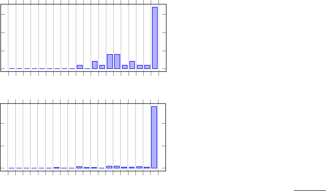
First we evaluated the embeddedness measure. Fig-

ure 3 shows histograms of embeddedness on the two

graphs. As we can observe from both histograms, val-

ues are strongly skewed towards 1, which suggests

that the majority of the vertices have connections only

inside their own communities. In fact, in the top-level

community structure in the Netscience network, ap-

proximately 98% of vertices have an embeddedness

equal to 1. As expected, the percent gets lower with

further decompositions of the community structure,

with 87% and 84% for levels 1 and 2 respectively, but

the distribution is still heavily skewed towards very

high values.

This highlights an important issue the embedded-

ness measure has: as was also observed in (Lanci-

chinetti et al., 2010; Orman et al., 2012), it appears

that in most real-world networks the majority of ver-

tices have connections only inside their own commu-

nities so the information conveyed by this measure

carries, in general, little meaning. Furthermore, if we

take for example the Karate network, the only connec-

tion of vertex 12 is inside its own community, so it has

an embeddedness of 1. Vertex 2 has 8 connections in-

side the community (to 75% of all vertices in the com-

munity) and one connection outside, so it has an em-

beddedness of 0.89. Intuitively however, one would

think that vertex 2 has a stronger commitment to the

community than vertex 12. The issue here is that em-

beddedness does not take the number (or indeed sum

of weights in a weighted network) of the connections

of a vertex into account, only the ratio between inter-

nal and external edges, which, while useful, does not

paint the whole picture.

Another issue with embeddedness can be ob-

served by looking at vertex 78 in level 2 of the

Assessing Vertex Relevance based on Community Detection

5 · 10

−2

0.1

0.15

0.2

0.25

0.3

0.35

0.4

0.45

0.5

0.55

0.6

0.65

0.7

0.75

0.8

0.85

0.9

0.95

Number of Vertices

5 · 10

−2

0.1

0.15

0.2

0.25

0.3

0.35

0.4

0.45

0.5

0.55

0.6

0.65

0.7

0.75

0.8

0.85

0.9

0.95

500

1,000

Embeddedness

Number of Vertices

Figure 3: Embeddedness histograms for the Karate network

(top) and level 2 of the Netscience network (bottom).

Netscience network. This vertex has an internal

weight of 16.25 and an external weight of 6.75 across

7 other communities. The embeddedness of this ver-

tex is 0.71, however the interior weight is far larger

than the weight towards any single other community.

Comparing the internal weight to the cumulative ex-

ternal weight creates a disadvantage for vertices who

are weakly connected to many other communities but

have a strong connection to their own community.

4.2 Signiﬁcance

Next, we have analyzed the vertices based on their

signiﬁcance. Instead of determining the signiﬁcance

clusters as done in (Rosvall and Bergstrom, 2010),

we have used the perturbation method described in

(Karrer et al., 2008) to determine a signiﬁcance mea-

sure for all vertices in the community structure of the

graph. The method we used is the following:

1. Generate a number (between 100 and 1000, more

on that later) of perturbed graphs with α = 0.2

(in every perturbed graph 20% of the edges were

moved).

2. Determine the community structure of each of

these perturbed graphs.

3. For each vertex, determine the percentage of per-

turbed graphs in which the vertex remained in the

same community as in the community structure of

the original graph.

The percentage computed in step 3 represents the

signiﬁcance of the vertex, based on the idea that ver-

tices which remain in the same community after the

graph is slightly perturbed have a high commitment

to that community.

The ﬁrst question that arises is how to determine

the corresponding communities of the same vertex in

two different community structures. This is necessary

in order to determine whether the vertex remained in

the same community or not after the graph was per-

turbed. To achieve this, we used the relative overlap

measure (Fortunato, 2010; Palla et al., 2007). Rel-

ative overlap (6) represents the number of vertices

shared between two communities, so in order to de-

termine the corresponding perturbed community we

choose the one with the highest relative overlap with

the original community.

i j

(6)

The next question we considered in the evalua-

tion process was how many perturbed graphs to gen-

erate? The authors of (Karrer et al., 2008) used a

number between 10 and 100, depending on the num-

ber of vertices of the network, while the authors in

(Rosvall and Bergstrom, 2010) used 1000 perturbed

graphs. The process of determining the signiﬁcance

of a vertex is non-deterministic, since the perturba-

tions applied to the graph have a random element (see

section 2.3). Since the signiﬁcance of a vertex is aver-

aged across all perturbed graphs, a higher number of

such graphs means a higher accuracy and reliability

in determining the measure, but also a higher com-

putation time because community detection has to be

performed for each of the perturbed graphs. Depend-

ing on the community detection algorithm used, this

can be rather computationally expensive. To deter-

mine what a good balance between accuracy and the

number of perturbed graphs would be, we calculated

the signiﬁcance of the vertices in both networks for

100, 250, 500, 750 and 1000 perturbed graphs. We

repeated each experiment 3 times and computed the

average standard deviation of the signiﬁcance values

(Figure 4).

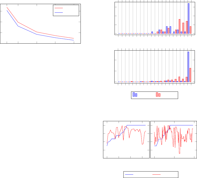
As can be noticed, the gains in accuracy be-

come smaller the more perturbed graphs are gener-

ated. Based on this observation we can conclude

that on these networks, 750 or even 500 perturbed

graphs provide a good trade-off between computation

time and accuracy. Another interesting observation

is that the standard deviation follows the same pat-

tern for both networks, although they have very dif-

ferent sizes. Even more, the standard deviation for

the larger network is consistently smaller than for the

smaller network. This suggests that for large net-

works a smaller number of perturbed graphs is suf-

KDIR 2015 - 7th International Conference on Knowledge Discovery and Information Retrieval

100

250 500 750

1,000

0.5

1.5

·10

−2

Number of perturbed graphs

Standard deviation

Karate

Netscience

Figure 4: Average standard deviation of signiﬁcance.

ﬁcient.

The signiﬁcance results presented next are for

1000 perturbed graphs. Figure 5 shows histograms

comparing signiﬁcance to embeddedness for both net-

works. We can observe that the distribution of signiﬁ-

cance is much more uniform, which suggests that this

measure does not suffer from the issue shown in sec-

tion 4.1. By comparing the two measures (Figure 6)

we cannot observe a signiﬁcant correlation between

them: vertices with high signiﬁcance do not neces-

sarily have high embeddedness or vice-versa. In-

deed, Pearson’s correlation coefﬁcient is r = 0.2 for

the Karate network and r = 0.01 for the Netscience

network. Since signiﬁcance essentially measures the

resilience of the membership of a vertex to pertur-

bations and considering these results and the issues

with embeddedness we have highlighted in section

4.1, signiﬁcance seems to be the better measure of the

two. We will be looking in more detail at the differ-

ences between embeddedness and signiﬁcance in the

following section.

5 NEW VERTEX MEASURES

In this section, we ﬁrst analyze the differences be-

tween signiﬁcance and embeddedness and identify

factors that inﬂuence signiﬁcance. Based on these

factors, we propose a new measure for commitment

called Relative Commitment. In section 5.2 we pro-

pose a method for assessing vertex importance by ob-

serving the effects of removing the vertex from the

graph and in section 5.3 we show how vertices can

be categorized based on measures of commitment and

importance.

5.1 Relative Commitment

As we determined earlier, signiﬁcance appears to be

the better measure for assessing commitment. How-

ever, it carries a drawback: a large processing time.

Depending on the desired accuracy, the graph has to

5 · 10

−2

0.1

0.15

0.2

0.25

0.3

0.35

0.4

0.45

0.5

0.55

0.6

0.65

0.7

0.75

0.8

0.85

0.9

0.95

Number of Vertices

5 · 10

−2

0.1

0.15

0.2

0.25

0.3

0.35

0.4

0.45

0.5

0.55

0.6

0.65

0.7

0.75

0.8

0.85

0.9

0.95

500

1,000

Number of Vertices

Embeddedness Signiﬁcance

Figure 5: Embeddedness and signiﬁcance histograms of the

Karate network (top) and the level 2 community structure

of the Netscience network (bottom).

0 10 20 30

0.2

0.4

0.6

0.8

Vertex Id

100

Vertex Id

Embeddedness Signiﬁcance

Figure 6: Embeddedness compared to signiﬁcance in the

Karate network (left) and the biggest community in the

Netscience network (right). Vertices are sorted in increasing

order of embeddedness.

be perturbed and community detection has to be per-

formed many times, while embeddedness is a simple

calculation which has to be performed once for each

vertex. It would be advantageous to have a measure

computed as fast as embeddedness, but which can

capture the information conveyed by signiﬁcance. To

this end, we investigated which other factors besides

the ratio between internal and external degree are im-

portant for the signiﬁcance, by looking at the differ-

ences between the signiﬁcance and the embeddedness

of vertices in the Karate network. We attempt to de-

ﬁne an improved measure based on our ﬁndings.

The ﬁrst issue we identiﬁed with embeddedness is

that it does not take the internal degree of the ver-

tex into account, only its ratio to the total degree,

which can be misleading. So, as a ﬁrst improve-

ment to embeddedness we considered using the rela-

Assessing Vertex Relevance based on Community Detection

tive internal degree rk

of the vertex: k

/Max

where k

represents the internal degree of vertex

i and Max

) is the maximum internal degree in

community s. However, we observed that vertices

with a medium number of internal connections had

a score that was too low and thus we applied the loga-

rithmic formula in equation (7). In a weighted graph,

we can use the relative internal weight rw

, where

we replace the internal degree with internal weight in

equation (7).

log(k

+ 1)

log(Max

) + 1)

(7)

We also observed that there are vertices with a

relatively small number of connections, but with a

high signiﬁcance. Looking at those vertices we re-

alized that they were connected to other vertices in

the same community that had a high internal degree,

so they were less likely to leave the community when

the graph was perturbed. A good example is vertex

15 in the Karate network which has only two connec-

tions in its community, so judging solely by relative

internal degree (considering that the maximum inter-

nal degree in that community is 14) one would think it

has a weak connection to the community. The signiﬁ-

cance of vertex 15 is however high at 0.9, most likely

because it is connected to the two most connected ver-

tices in the community: 33 and 34. Considering this,

it seems natural that not only the internal degree, but

also the internal neighborhood (neighbors within the

community) of the vertex is an important factor for its

connection strength. It is important to note that the

internal neighborhood should only have a positive ef-

fect on the score of the vertex: a well-connected ver-

tex should not have its score lowered simply because

it is connected to low-degree vertices.

Similar to the previous point, we found that we

also have to look at the external neighborhood of a

vertex: a vertex that is well connected inside its own

community but has connections with well-connected

vertices in other communities will have a higher like-

lihood of leaving the community. A good example for

such a vertex is 32: it has an internal degree of 5, an

external degree of only 1 and is connected to vertices

33 and 34, so one would expect a high signiﬁcance.

The signiﬁcance is actually quite low, at 0.63, because

it is connected to vertex 1, which is the most con-

nected vertex in another community. One can view

highly connected vertices as attractors that exercise a

pulling force on their weaker-connected neighbors, so

neighbors both inside and outside of the community

have to be considered.

To summarize, we have identiﬁed the following

factors which should be considered for estimating

how strongly a vertex belongs to its own community

(i.e. measuring commitment):

• The internal degree

• The internal degree of its internal neighbors

• The internal degree of its external neighbors

Considering the fact that embeddedness does not

represent a sufﬁciently expressive metric for estimat-

ing the commitment of a vertex, and that signiﬁcance

is computationally intensive, we propose a new mea-

sure for quantifying vertex commitment, which we

call Relative Commitment. We deﬁne the internal

score of a vertex to be the sum of the relative inter-

nal degrees of its internal neighbors and the external

score, the sum of the relative internal degrees of its

external neighbors. Relative Commitment is the ratio

between the internal score and the total score (internal

+ external), multiplied by the relative internal degree

of the vertex in question. Thus, we obtain the formula

in equation (8), where rk

represents the relative in-

ternal degree of the vertex and i and j denote the inter-

nal and external neighbors of the vertex, respectively.

rc = rk

∗

∑

(8)

For a weighted graph, we use relative internal

weight instead of degree and additionally we use the

connection weight to each neighbor in the internal

and external score (9), where w

and w

represent the

weight of the connection with internal neighbor i and

external neighbor j, respectively.

rcw = rw

∗

∑

∗ rw

∑

∗ rw

∑

∗ rw

(9)

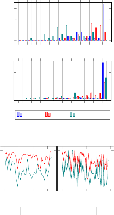
Figure 7 shows histograms comparing the Relative

Commitment to embeddedness and signiﬁcance for

both Karate and Netscience networks. In the Karate

network the Relative Commitment values are on aver-

age lower than signiﬁcance, while in the Netscience

network, we have more values of Relative Commit-

ment between 0.95 and 1.0.

Figure 8 shows Relative Commitment compared

to signiﬁcance for both networks. As we can see,

there is a clear correlation between the two measures

for many vertices. For both networks, the correlation

coefﬁcient r is approximately 0.59. This means that

the factors identiﬁed previously are indeed important

for the signiﬁcance of the vertices. However, we can

see that there are still differences, vertices that have

a high Relative Commitment but a low signiﬁcance or

vice-versa, so there are still aspects of signiﬁcance we

have not covered in Relative Commitment. Still, even

in its current form, Relative Commitment represents a

KDIR 2015 - 7th International Conference on Knowledge Discovery and Information Retrieval

5 · 10

−2

0.1

0.15

0.2

0.25

0.3

0.35

0.4

0.45

0.5

0.55

0.6

0.65

0.7

0.75

0.8

0.85

0.9

0.95

Number of Vertices

5 · 10

−2

0.1

0.15

0.2

0.25

0.3

0.35

0.4

0.45

0.5

0.55

0.6

0.65

0.7

0.75

0.8

0.85

0.9

0.95

500

1,000

Number of Vertices

Embeddedness Signiﬁcance Relative Commitment

Figure 7: Embeddedness, signiﬁcance and Relative Com-

mitment histograms for the Karate network (top) and level

2 of the Netscience network (bottom).

0 10 20 30

0.5

Vertex Id

100

Vertex Id

Signiﬁcance Relative Commitment

Figure 8: Signiﬁcance compared to Relative Commitment

in the Karate network (left) and the biggest community in

the Netscience network (right).

good approximation of signiﬁcance and can be used

in cases where the processing time of signiﬁcance is

an impediment.

5.2 Vertex Importance

In addition to analyzing the commitment of vertices,

we wanted to assess the importance of a vertex by

looking at what happens to the community structure

if that vertex is removed from the graph. Based on

the idea that the more important a vertex is, the larger

the disruption caused will be, idea supported by the

ﬁndings in (Albert et al., 2000), we propose the fol-

lowing method of assessing vertex importance:

1. Remove vertex from graph

2. Determine community structure in this graph

3. Compute the difference between the original com-

munity structure and the new community structure

Steps 1 and 2 are straightforward. Step 3 involves

measuring the disruption the removal of the vertex

causes. In order to do this, we compute the normal-

ized version of the Variation of Information measure

deﬁned in equation (5). When computing Variation of

Information, we remove the vertex from the original

community structure and then compare it to the new

community structure. There are two different types

of disruption of interest: the disruption caused to the

community of the vertex (community disruption) and

the disruption caused to the community structure as

a whole (community structure disruption). From the

standpoint of determining the importance of the ver-

tex for its own community, community disruption is

relevant. But, as we will see, community structure

disruption can also convey useful information.

The same method described above can be easily

applied on edges, to determine the most important

edges in a community. We will analyze vertices of the

Karate network using both vertex and edge omission.

5.2.1 Vertex Omission

Figure 9 shows the result of applying the described

vertex omission method on the Karate network. As

expected, community disruption ≤ community struc-

ture disruption. We can observe that disruption seems

to have a weak negative correlation with embedded-

ness: vertices with low embeddedness tend to have

non-zero disruption values. Community disruption

has a correlation coefﬁcient r = −0.14 while for com-

munity structure disruption r = −0.29. At ﬁrst im-

pression, it might seem that vertices that have em-

beddedness < 1 should cause community structure

disruption since they have both internal and external

edges. However, the negative correlation also appears

to hold for community disruption, where the disap-

pearance of external edges should have no negative

impact on the community. It is possible that vertices

with connections both inside and outside the commu-

nity tend to be the most inﬂuential.

We note that disruption does not seem to be cor-

related with signiﬁcance (r = 0.09 and r = 0.16 for

community and community structure disruption, re-

spectively). There are vertices with high signiﬁcance

and no disruption, and there are vertices with low sig-

niﬁcance but whose removal disrupts the community.

At ﬁrst glance, this represents a surprising result: one

would expect the removal of the most signiﬁcant ver-

tices to be the most disruptive. However, after looking

at the vertices in these networks we can conclude the

following: measures like embeddedness, signiﬁcance

Assessing Vertex Relevance based on Community Detection

0 10 20 30

0.5

Vertex Id

Embeddedness Signiﬁcance

Comm. Disruption Comm. Structure Disruption

Figure 9: Disruption compared to embeddedness and sig-

niﬁcance for the Karate network. Vertices are sorted in in-

creasing order of embeddedness.

and Relative Commitment measure the commitment

of a vertex to a community, the strength of the mem-

bership of that vertex. Disruption on the other hand

measures how important the vertex is for the structure

of the community. To elaborate on this, let us analyze

vertices in the Karate network.

Vertex 4 has a very high signiﬁcance of 0.97 but

a community disruption of 0. This means that, upon

removing the vertex, nothing changed in the commu-

nity. Whether the vertex exists or not, the commu-

nity remains unchanged. Its high signiﬁcance how-

ever suggests that its membership is resilient to per-

turbations, which makes sense given that it has 6 in-

ternal connections and no external connections. So

this vertex is a very good representative of a vertex

that has a strong membership to its community but a

low importance for the structure of that community.

Another relevant example is vertex 32, which has

a very low signiﬁcance (0.56), but a quite high com-

munity disruption (0.09). As discussed previously, its

signiﬁcance is low probably because of its connec-

tion with a well-connected vertex in another commu-

nity. Removing the vertex causes its community to

split, which indicates that the vertex is important to

the structure of the community. The commitment of

vertex 32 to its own community is not very strong, but

its existence keeps the community together.

There are vertices, such as 34 or 33, which have

both high signiﬁcance and high disruption. Of course,

some vertices, such as 25, have both low commitment

and low importance to their own communities.

5.2.2 Edge Omission

We applied the same omission method described pre-

viously to the edges of the Karate network in order

to measure their importance. As we can observe in

Figure 10, the edges of highly relevant vertices such

as 24, 33 and 34 are also important. However, there

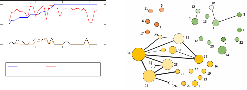
Figure 10: The Karate network: vertex color intensity is

proportional to signiﬁcance, vertex size is proportional to

vertex community disruption and edge width is proportional

to edge community disruption.

are vertices with non-zero disruption such as 14, 15

and 16 whose connections have no disruption. What

this tells us is that the removal of the edges of these

vertices as a whole has an impact on the community,

and not the removal of individual edges.

5.3 Vertex Categorization

We propose a generic categorization of vertices into

4 categories based on their commitment and impor-

tance (Table 1). We use signiﬁcance and community

disruption, but in theory, any measures that quantify

commitment and importance can be used to catego-

rize vertices.

We proceeded and categorized the vertices in the

Karate network based on these criteria. We consider

signiﬁcance to be high if it is ≥ 0.75 and low if it

is < 0.75. For community disruption, we consid-

ered vertices with 0 disruption to have low impor-

tance, while the rest have high importance. Similar to

our categorization, Guimera and Amaral describe in

(Guimera and Amaral, 2005) a way to assign univer-

sal roles to vertices based on their z-score and partic-

ipation coefﬁcient. Table 2 shows our categorization

compared to the universal roles of these vertices.

We can observe that a few of the vertices fall into

category I, which means they are the most relevant for

their respective communities. A single vertex falls in

category II: 32, which has high importance but low

commitment. Most vertices fall in category III, which

is consistent with our expectations of social networks:

we expect most vertices to have a good commitment

to their own communities, especially since most ver-

tices don’t have external connections, and their im-

portance to be low. We also have a few category IV

vertices, which are the least relevant.

KDIR 2015 - 7th International Conference on Knowledge Discovery and Information Retrieval

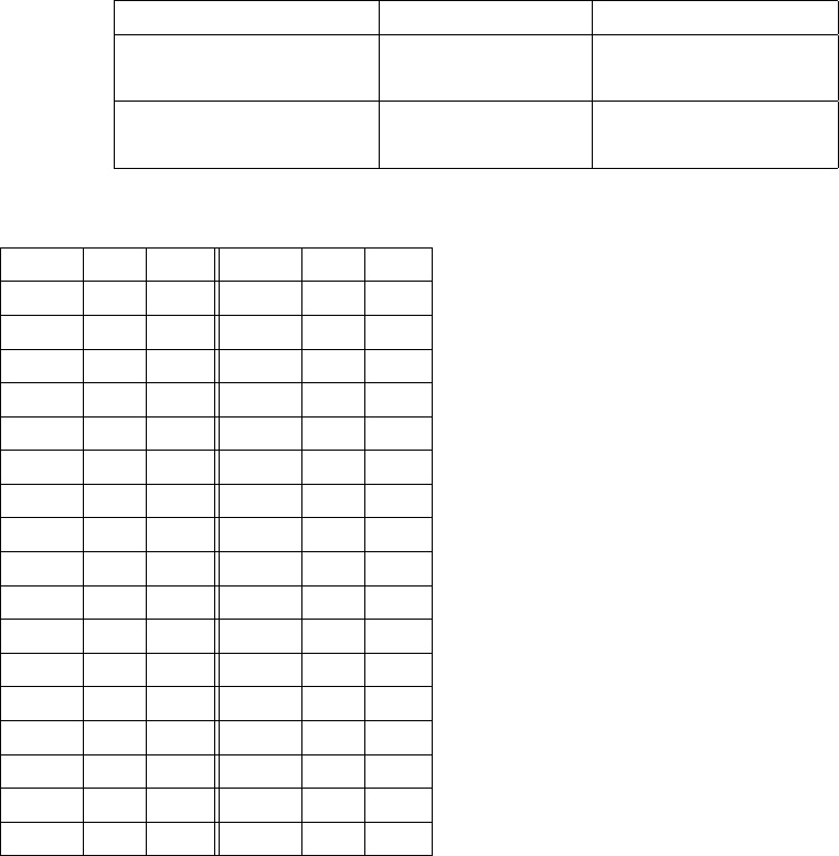
Table 1: Vertex Categories.

Commitment \ Importance High Low

High

Category I:

highly relevant

Category III: committed,

but unimportant

Low

Category II: relevant,

but uncommitted

Category IV:

irrelevant

Table 2: Categories and roles for vertices in the Karate net-

work.

Vertex Cat. Role Vertex Cat. Role

1 I R2 18 III R1

2 III R2 19 III R1

3 I R2 20 III R2

4 III R1 21 III R1

5 III R2 22 III R1

6 III R2 23 III R1

7 III R2 24 I R1

8 III R1 25 IV R1

9 III R2 26 IV R1

10 IV R2 27 III R1

11 III R2 28 II R2

12 IV R1 29 IV R2

13 III R1 30 III R1

14 I R2 31 I R2

15 I R1 32 II R2

16 I R1 33 I R2

17 III R1 34 I R5

Now let us look at how the universal roles com-

pare to our categories. The vertex with both the high-

est signiﬁcance and importance, 34, is the only hub

and has the “provincial hub” role (R5). Other highly

relevant vertices like 1 and 33 can be promoted to

the R5 role by lowering the z-score threshold, but all

other vertices have either “ultra-peripheral” or “pe-

ripheral” roles (R1 and R2): they have no or very few

external connections so the participation coefﬁcient

tends to be low. Aside from category I vertices, there

does not seem to be a clear correspondence between

our categories and the universal roles, since both pe-

ripheral and ultra-peripheral vertices can have varying

degrees of importance and commitment. One more

thing to note is that since the universal roles are based

on z-score and participation coefﬁcient, two measures

that quantify vertex commitment, they do not take im-

portance into consideration.

Another interesting observation is the relationship

between the community disruption and community

structure disruption of a vertex. As noted before,

community structure disruption ≥ community disrup-

tion and based on the behavior observed in the Karate

network, we can draw the following conclusions:

• If community disruption > 0 and community

disruption = community structure disruption, it

means that upon removal, the community of the

vertex decomposed into sub-communities, the

other communities remaining unaffected.

• If community disruption < community structure

disruption, it means that other communities were

affected by the removal of the vertex and either

lost or gained vertices.

6 CONCLUSIONS

This paper investigates different measures for quanti-

fying the relevance of a vertex in its own community.

We identiﬁed two related, but distinct vertex proper-

ties: commitment and importance. Commitment indi-

cates how strongly a vertex belongs to its own com-

munity, while importance shows how relevant a ver-

tex is to that community’s structure. We found that

embeddedness, although easy to compute, does not

carry much information and that signiﬁcance is better

as a measure for capturing the commitment of a ver-

tex. By comparing signiﬁcance and embeddedness,

we identiﬁed that not only the number of connections

of a vertex is important to its commitment, but also

to which other vertices it is connected to. Based on

this, we were able to propose a new measure, Relative

Commitment, which provides a more accurate estima-

tion of a vertex commitment than embeddedness, yet

is easier to compute than signiﬁcance.

By removing a vertex from its graph and observ-

ing the changes inside its community and outside (in

the overall community structure), we were able to as-

sess the importance of the vertex, which we identiﬁed

as a distinct property to embeddedness. We show that

this strategy is also applicable to edges, to assess their

individual importance.

The community structure of a network offers

much information on the relevance of a vertex. By

Assessing Vertex Relevance based on Community Detection

looking at commitment and importance, the most rel-

evant vertices in a community can be identiﬁed. To

this end, we proposed a vertex categorization strat-

egy, based on commitment and importance. Knowing

which are the relevant vertices in a network is partic-

ularly of interest in large networks, where extracting

meaningful information is difﬁcult. Potential appli-

cation areas for our methods include social networks,

in which group leaders and inﬂuential people can be

identiﬁed, or professional networks - determining the

best candidates for hiring. These measures also pro-

vide answers to questions about why a community ex-

ists and what is keeping vertices from leaving a spe-

ciﬁc community and joining another one.

We are currently focusing on further investigat-

ing the differences between embeddedness and sig-

niﬁcance in order to identify other factors which in-

ﬂuence the latter. These factors can then be used to

improve the Relative Commitment measure. It would

also be useful to extend the evaluation of these mea-

sures to other types of networks. Alternative, less

computationally intensive measures for assessing ver-

tex importance should also be studied, since vertex

disruption requires the community structure to be re-

computed for each vertex removal.

REFERENCES

Albert, R., Jeong, H., and Barabasi, A. L. (2000). Error

and attack tolerance of complex networks. Nature,

406(6794):378–382.

Fortunato, S. (2010). Community detection in graphs.

Physics Reports, 486(3-5):75–174.

Fortunato, S. and Castellano, C. (2008). Community struc-

ture in graphs. In Encyclopedia of Complexity and

Systems Science, pages 1141–1163.

Guimera, R. and Amaral, L. A. N. (2005). Cartography of

complex networks: modules and universal roles. Jour-

nal of Statistical Mechanics: Theory and Experiment,

2005(P02001):P02001–1–P02001–13.

Karrer, B., Levina, E., and Newman, M. E. J. (2008). Ro-

bustness of community structure in networks. Phys.

Rev. E, 77:046119.

Lancichinetti, A. and Fortunato, S. (2009). Community de-

tection algorithms: a comparative analysis. Phys. Rev.

E, 80:056117.

Lancichinetti, A., Kivela, M., Saramaki, J., and Fortunato,

S. (2010). Characterizing the community structure of

complex networks. CoRR, abs/1005.4376.

Newman, M. E. J. (2003). The structure and function of

complex networks. SIAM REVIEW, 45:167–256.

Newman, M. E. J. (2004). Fast algorithm for detect-

ing community structure in networks. Phys. Rev. E,

69:066133.

Newman, M. E. J. (2006). Finding community structure in

networks using the eigenvectors of matrices. Physical

review E, 74(3).

Orman, G. K., Labatut, V., and Cheriﬁ, H. (2012). Compar-

ative evaluation of community detection algorithms:

A topological approach. Journal of Statistical Me-

chanics: Theory and Experiment, P08001.

Palla, G., Barabasi, A. L., and Vicsek, T. (2007). Quanti-

fying social group evolution. Nature, 446(7136):664–

667.

Rosvall, M. and Bergstrom, C. T. (2008). Maps of random

walks on complex networks reveal community struc-

ture. Proceedings of the National Academy of Sci-

ences, 105(4):1118–1123.

Rosvall, M. and Bergstrom, C. T. (2010). Mapping change

in large networks. PLoS ONE, 5(1):e8694.

Zachary, W. W. (1977). An information ﬂow model for con-

ﬂict and ﬁssion in small groups. Journal of Anthropo-

logical Research, 33:452–473.

KDIR 2015 - 7th International Conference on Knowledge Discovery and Information Retrieval