Gaussian Nonlinear Line Attractor for Learning Multidimensional Data

Theus H. Aspiras

, Vijayan K. Asari

and Wesam Sakla

Department of Electrical and Computer Engineering, University of Dayton, U.S.A.

Air Force Research Laboratory, Wright Patterson Air Force Base, U.S.A.

Keywords:

Nonlinear Line Attractor, Multidimensional Data, Neural Networks, Machine Learning.

Abstract:

The human brain’s ability to extract information from multidimensional data modeled by the Nonlinear Line

Attractor (NLA), where nodes are connected by polynomial weight sets. Neuron connections in this archi-

tecture assumes complete connectivity with all other neurons, thus creating a huge web of connections. We

envision that each neuron should be connected to a group of surrounding neurons with weighted connection

strengths that reduces with proximity to the neuron. To develop the weighted NLA architecture, we use a

Gaussian weighting strategy to model the proximity, which will also reduce the computation times signiﬁ-

cantly. Once all data has been trained in the NLA network, the weight set can be reduced using a locality

preserving nonlinear dimensionality reduction technique. By reducing the weight sets using this technique,

we can reduce the amount of outputs for recognition tasks. An appropriate distance measure can then be used

for comparing testing data and the trained data when processed through the NLA architecture. It is observed

that the proposed GNLA algorithm reduces training time signiﬁcantly and is able to provide even better recog-

nition using fewer dimensions than the original NLA algorithm. We have tested this algorithm and showed

that it works well in different datasets, including the EO Synthetic Vehicle database and the Shefﬁeld face

database.

1 INTRODUCTION

Much research work has been done on modeling brain

functions and activities. The brain has around 10

neurons and each neuron has up to ten thousand

synaptic connections to other neurons around it. The

brain has a unique ability to utilize groups of these

neurons to formulate different lobes and structures to

regulate bodily functions, emotional responses, and

even cognition. All of these structures are able to

unify together to handle numerous inputs from the

different senses and have the ability to respond simul-

taneously.

When developing neurons and synaptic weights

of the brain, models for these must have a set struc-

ture, an ability for ﬁring/nonﬁring of neurons through

the synaptic junctions, training of the structure, and

continuous training of the system. Artiﬁcial neural

networks are the most explored models of the hu-

man brain, which encompass different modeling tech-

niques of the brain. One area of neural networks is

the recurrent neural network, which are able to send

outputs to the same stage of the network. This type

of neural network is also called an attractor network,

which attracts towards a certain pattern. In this paper,

we will be exploring attractor networks and how to

improve them.

1.1 Attractor Neural Networks

There are different types of attractor networks which

can model different dynamics of networks. One type

is the ﬁxed point attractor, which is the Hopﬁeld net-

work (Hopﬁeld, 1982). Given an underlying energy

function for minimization, the network asymptoti-

cally approaches a desired state. These networks are

associative, meaning that they can approach towards a

speciﬁc state given only part of the data. Other types

include the cyclic attractor networks to govern oscil-

latory behaviors (Lewis and Glass, 1991). The type

we will be focusing on is the line attractor (Zhang,

1996).

Line attractor networks work well for states that

are not just a speciﬁc point but a line of points. Point

attractor networks disregard any ability to attract to

a speciﬁc trained image of a class, unless there are

multiple point attractors for one class. Line attrac-

tor network assume continuity between data points,

which allows an estimation of data points that are

not fully trained in the dataset. Since manifolds in

130

Aspiras, T., Asari, V. and Sakla, W..

Gaussian Nonlinear Line Attractor for Learning Multidimensional Data.

In Proceedings of the 7th International Joint Conference on Computational Intelligence (IJCCI 2015) - Volume 3: NCTA, pages 130-137

ISBN: 978-989-758-157-1

a high-dimensional space are usually nonlinear, it is

best to incorporate a nonlinear line attractor to model

the manifold in space. Thus in this paper, we utilize

the nonlinear line attractor (NLA) network as the sup-

porting architecture for our work.

1.2 Biological Implications

With the use of recurrent associative networks, most

are totally interconnected, meaning that every node is

connected to all other nodes. This type of architec-

ture allows inﬂuence of all nodes, especially if there

are signiﬁcant changes in input at farther nodes. But

in biological structures, nodes are only interconnected

with surrounding nodes with longer, weaker connec-

tions with farther nodes. These types are expressed

by Tononi et al. (Tononi et al., 1999), who found that

there is much redundancy in highly interconnected

networks. They introduced an optimized degenera-

tive case, which minimizes the amount of connections

while maintaining the cognitive ability and reducing

redundancy.

By using only neighborhood connections, por-

tions of the network will be responsible for model-

ing that region while relying on the propagation of

inﬂuence from other sections to travel as the network

iterates. This local modeling will aid in faster conver-

gence due to reliance to only closer nodes and give

way to higher variance areas, which contain more in-

formation than other areas of input, for example a

background region. This also reduces the amount of

redundancies in the network for modeling a speciﬁc

portion of data. Guido et al. (Guido et al., 1990)

found that there is functional compensation when the

visual cortex, which is highly modular, is damaged.

1.3 Modularity in Neural Networks

By developing neighboring connections, we can cre-

ate modularity while still keeping inter-connectivity

in the networks. Happel et al. (Happel and Murre,

1994) investigated various interconnections and mod-

ularity in networks and found that different conﬁgu-

rations aided in further recognition of different tasks.

Other techniques also used modularity, like modu-

lar principal component analysis (Gottumukkal and

Asari, 2004), which takes speciﬁc portions of an im-

age and takes the PCA of those sub-images to aid in

the recognition of the whole image. Modularity re-

duces the model complexity which uses speciﬁc mod-

ules to learn only a portion of data to aid in the overall

complex task (Gomi and Kawato, 1993).

Instead of fully incorporating modularity, algo-

rithms also include overlap between modules to im-

prove the recognition capabilities. Auda et al. (Auda

and Kamel, 1997) used Cooperative Modular Neural

Networks with various degrees of overlap to improve

various classiﬁcation applications. Also since mod-

ularity reduces the amount of connections between

neurons by dividing processing into smaller subtasks,

the amount of computations can be greatly reduced.

The type of neural network we will be looking at

is the nonlinear line attractor, proposed by Seow et

al. (Seow and Asari, 2004), which has been used for

skin color association, pattern association (Seow and

Asari, 2006), and pose and expression invariant face

recognition (Seow et al., 2012). Given that modu-

larity is able to reduce computation complexity and

improve recognition in many cases, we aim to incor-

porate it into the nonlinear line attractor network. In-

stead of complete modularity, we propose a smooth,

Gaussian weighting strategy to make smooth overlaps

for each module. According to the weighting scheme

of the network, modularity will also reduce the com-

plexity of the modeling of the network. In (Seow

et al., 2012), the weighting scheme is reduced using

Nonlinear Dimensionality Reduction. We will look

into the ability of the algorithm to reduce the weights

and propose an improvement to the algorithm.

The main contributions of this paper are:

• Gaussian weighting strategy to the Nonlinear Line

Attractor Network to introduce modularity

• Reduction of the computational complexity to im-

prove the convergence time of the GNLA archi-

tecture

• An improved scenario for using the Nonlinear Di-

mensionality Reduction for object recognition

2 METHODOLOGY

The nonlinear line attractor network is a recurrent as-

sociative neural network, which aims to converge on

a trained pattern given an input. Each trained pat-

tern has connective information, which links one de-

gree of information to another. These trained patterns

usually are learned as a point in the feature space

and thus variations of the pattern would be repre-

sented as a basin. Convergence would specify that

the input pattern would be associated to one of the

learned patterns. When considering a basin of attrac-

tion, single point representations of a particular set

of patterns may be insufﬁcient to totally encompass

the patterns. The NLA architecture formulates a non-

linear line representation which would allow patterns

to converge towards the line attractor. An example

would be using manifold learning on a set of objects

Gaussian Nonlinear Line Attractor for Learning Multidimensional Data

131

with varying poses. As the poses move in the high-

dimensional space, the manifold would form a non-

linear line, which would be best modeled by the NLA

architecture.

Let the response x

of the i

neuron due to the

excitations x

from other neurons for the s

pattern

in a fully connected recurrent neural network with n

neurons be expressed as:

(i,s)

∑

j=1

( j,s)

) for 1 ≤ i ≤ N (1)

where Λ

is deﬁned by a k

order nonlinear line

as:

( j,s)

) =

∑

m=0

(m,i j)

( j,s)

)

for 1 ≤ i, j ≤ N (2)

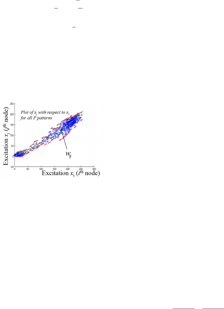
This equation deﬁnes a polynomial best ﬁt line to

encompass all input/output pairs given from each pat-

tern s. The green line in Figure 1 shows this best ﬁt

line. The m

order term of the resultant memory w

can be expressed as:







(m,11)

. . . w

(m,1N)

(m,N1)

. . . w

(m,NN)







for 0 ≤ m ≤ k

(3)

The weights are in matrix form to show a fully

interconnected weight system. Since the input and

output have the same number of nodes due to the as-

sociative nature of the algorithm, we can show these

weights in this regard. To calculate the weights, we

can use error descending characteristics. The least

squares estimation approach is able to calculate the

best ﬁt line using the polynomial method. To mini-

mize the least squares error in the weight matrix, we

can formulate the following equation, which yields

the optimum weight set.

i j

(0,i j)

(1,i j)

, ..., w

(k,i j)

] =

∑

s=1

(i,s)

− Λ

( j,s)

)]

for 1 ≤ s ≤ P

(4)

To minimize the least squares error, we must

equate the derivative of the error with respect to the

weight to be zero, as shown in the following equation.

δE

i j

δw

(m,i j)

= 0 for each m = 0, 1, . . . , k (5)

We can then ﬁnd that the equation can be reduced

to a set of linear equations based on the order of the

polynomial, as shown below.

(0,i j)

∑

s=1

( j,s)

)

+ w

(1,i j)

∑

s=1

( j,s)

)

+ . . .

+ w

(k,i j)

∑

s=1

( j,s)

)

∑

s=1

(i,s)

( j,s)

)

(0,i j)

∑

s=1

( j,s)

)

+ w

(1,i j)

∑

s=1

( j,s)

)

+ . . .

+ w

(k,i j)

∑

s=1

( j,s)

)

k+1

∑

s=1

(i,s)

( j,s)

)

(0,i j)

∑

s=1

( j,s)

)

+ w

(1,i j)

∑

s=1

( j,s)

)

k+1

+ . . .

+ w

(k,i j)

∑

s=1

( j,s)

)

∑

s=1

(i,s)

( j,s)

)

(6)

Given that there is a nonlinear line that models

the relationship between inputs, as modeled by the

trained weight sets, there must be another modeling

of the variances of the data. This is done by creating

an activation function, as shown in equation 7.



Λ[x

(t + 1)]













(t) if ψ

(i j,−)

≤ {Λ

(t + 1) − x

(t + 1)}

≤ ψ

(i j,+)

(t + 1)] otherwise

(7)

where

(t)) =

∑

m=0

(m,i j)

(t))

(8)

An activation function can be used to see if a data

point that runs through the system is trained into the

manifold. Since data points do not exactly ﬁt in the

best ﬁt nonlinear line, thresholds [ψ

(i j,−)

, ψ

(i j,+)

] are

created to ensure that data points do not update if

the estimated data point lies within the manifold. If

the data point falls away from the manifold, the best

ﬁt equation can be used to attract the data point to-

wards the manifold. These threshold regions can be

expressed as:

(i j,−)











(1,i j,−)

if 0 ≤ x

Ω

(2,i j,−)

Ω

≤ x

Ω

(Ω,i j,−)

if (Ω − 1)

Ω

≤ x

< L

(9)

NCTA 2015 - 7th International Conference on Neural Computation Theory and Applications

132

(i j,+)











(1,i j,+)

if 0 ≤ x

Ω

(2,i j,+)

Ω

≤ x

Ω

(Ω,i j,+)

if (Ω − 1)

Ω

≤ x

< L

(10)

where L is the number of segments used for the

piecewise threshold regions and Ω is the length of the

manifold. When using a nonlinear dimensionality re-

duction technique, as shown in a further section, the

threshold regions created will not be used, due to the

nonlinear line attractor becoming a transform from

the original image space to a reduced dimensionality

space. Figure 1 shows how the weights are intercon-

nect through the inputs.

Figure 1: Interconnection of Weights. The green line cap-

tures the nonlinear line modeling and the red lines capture

the variances of the data.

Since this is modeling of a speciﬁc manifold, mul-

tiple manifolds may be needed to encompass more

of a class. Most will require a speciﬁc manifold per

class, so there will be at least one weight set per class.

2.0.1 Computational Strategy

We have devised an effective computational strategy

for training data. Given equation 6, previous mod-

els of the computational strategy require computing

powers for each interconnection, in which there are

several calculations that are repeated in the equations

while traversing through each interconnection. In-

stead of having redundant calculations, we can divide

the weight calculation into different steps.

Stage 1 would be the calculation of powers for the

inputs. In equation 6, we see that every x

has an order

associated with it. Calculation of these terms would

be redundant for all different combinations of inputs

and outputs, since there are multiple terms with the

same order, hence the same value. Computing only

the powers in this stage would tremendously reduce

the computation time of the system.

Stage 2 would be the calculation of the weights,

given the set of normal equations and using the val-

ues obtained from stage 1. The solving of the nor-

mal equations can be done using a linear solve al-

gorithm. This stage will take a considerable amount

of time due to the volume of data, speciﬁcally the

number of inputs, since the weight matrix size is

#inputs × #inputs × order where # inputs refer to the

size of the image.

Stage 3 would be the calculation of the activa-

tion function, which will also require a considerable

amount of computation time. Since the computa-

tion of the orders for all of the input data are already

known, the activation function can be formulated us-

ing that data.

Stage 4 would be the calculation of the nonlinear

dimensionality reduction. This step would require all

of the weights and is dependent on the number of in-

puts and also the order of the weight system.

2.1 Gaussian Nonlinear Line Attractor

(GNLA) Network

The Gaussian Nonlinear Line Attractor Network is a

modiﬁcation to the original NLA network, which uses

a neighborhood approach to improve the algorithm.

Local information is more important than distant in-

formation, when looking from a biological perspec-

tive, so it can be assumed that using this architecture

for the NLA algorithm would improve run times and

classiﬁcation ability. When dealing with imagery, a 2-

dimensional spatial relationship is created with each

node. By incorporating this spatial relationship into

the nodes, we can increase the recognition while re-

ducing computation time.

When implementing a Gaussian neighborhood ap-

proach, we can change the coefﬁcient in the front and

add the distance equation. The equation can then be

modiﬁed as:

(i,s)

∑

j=1

i j

( j,s)

) for 1 ≤ i ≤ N (11)

where

i j

= exp

−

( ˆx

− ˆx

)

2σ

ˆx

( ˆy

− ˆy

)

2σ

ˆy

(12)

For these equations, ˆx and ˆy deﬁne the spatial co-

ordinates of the input x. Instead of using the Gaus-

sian function, we can use the Gaussian kernel , for

example a 13x13 Gaussian kernel as shown in Figure

2. This will effectively reduce the computation time.

We can then change the equation as

Gaussian Nonlinear Line Attractor for Learning Multidimensional Data

133

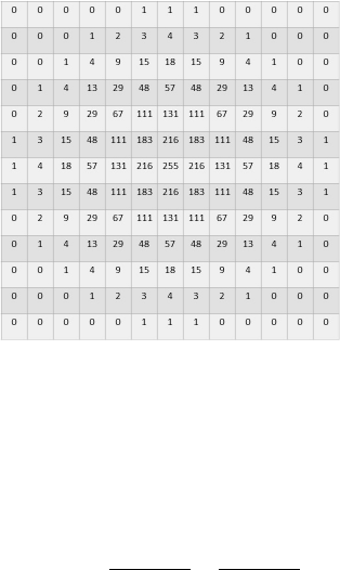
Figure 2: An example of a 13 x 13 Gaussian kernel.

(i,s)

∑

j=1

i j

( j,s)

) for 1 ≤ i ≤ N (13)

Where n is the size of the kernel and A

i j

= exp

−

( ˆx

− ˆx

)

2σ

ˆx

( ˆy

− ˆy

)

2σ

ˆy

(14)

We can also effectively reduce the computation

time of the kernel by not computing any portion that

contains zeros. According to the Gaussian kernel

above (which is a 13x13), roughly 28% of the Gaus-

sian kernel are zeros, thus a reduction of the computa-

tion time can be accomplished by ignoring those com-

putations.

2.1.1 Nonlinear Dimensionality Reduction

To reduce the size of the weight sets, we can reduce

the dimensionality of the weights. Since the weights

obtained through training have embedded the mani-

folds, we can use the weights in the reduction process.

Given that there are r different line attractor networks,

there will be y different outputs, as shown in the fol-

lowing equation.

= W

1,k

1,k−1

k−1

+ ··· +W

1,0

= W

2,k

2,k−1

k−1

+ ··· +W

2,0

= W

r,k

r,k−1

k−1

+ ··· +W

r,0

(15)

Previous algorithms of the Nonlinear Line Attrac-

tor use singular value decomposition (SVD) (Golub

and Reinsch, 1970) to reduce the weight set. We pro-

pose using a different strategy to reduce the weight

set. Given that the locally linear embedding (LLE)

(Roweis and Saul, 2000) algorithm contains intercon-

nected weight sets for different datapoints, we can use

that strategy to reduce the weights of the NLA net-

work.

Each m

term of the networks’ memory is evalu-

ated using the LLE algorithm. We ﬁrst obtain a sparse

matrix M using the following equation.

(m,d)

=(I − w

(m,d)

)

∗ (I − w

(m,d)

)

for 0 ≤ m ≤ k; 1 ≤ d ≤ r

(16)

We then take the smallest z eigenvectors from

M and use them as the projection into the lower-

dimensional subspace. The projection of the N-

dimensional data to a z-dimensional subspace using a

z × N sub-matrix obtained from the smallest z eigen-

vectors of the LLE yields a z-dimensional output Y

where z << N. Once the lower-dimensional subspace

is obtained, we can then use an appropriate distance

measure, like Euclidean distance, to ﬁnd the closest

match of a test image to the trained images in the sys-

tem.

When calculating the weight matrices for the

Gaussian NLA network, none of the weights contain

any information of the Gaussian distances. To incor-

porate the function inside the weights, we must embed

the terms into the weights by multiplying the normal-

ized mask with the weights. Given equation 16, we

can embed the normalized coefﬁcients to multiply the

weights using the following equation.







(11)

. . . a

(1N)

(N1)

. . . a

(NN)







(17)

The resultant multiplication of the weight set is

given by the equation below.

¯w

(m,s)







¯w

(m,11,s)

. . . ¯w

(m,1N,s)

¯w

(m,N1,s)

. . . ¯w

(m,NN,s)







for 0 ≤ m ≤ k

(18)

This nonlinear dimensionality reduction tech-

nique using LLE computes each order of the weight

matrices separately. There is no interconnection be-

tween the orders, in which the original algorithm con-

tains a summation between the orders to results in the

ﬁnal outputs. We propose that instead of reducing this

dimensionality by adding the orders of the matrix for

the results, we can concatenate all of the orders, which

are multiplied by the input, to yield a larger vector

NCTA 2015 - 7th International Conference on Neural Computation Theory and Applications

134

without the reduction resulting from the summation.

This will allow even better recognition results using

fewer total weights, even though the resulting vector

can be potentially larger.

2.1.2 Complexity

In Stage 1, we can ﬁnd that it will be the same com-

plexity as the previous algorithm since we are just

computing the powers.

In Stage 2, the original complexity is #inputs ×

#inputs × order

due to the linear solve algorithm,

but modiﬁed complexity is #inputs × #neighbors ×

order

, where # neighbors is signiﬁcantly smaller

than the size of the network. For example, given that

we have a network of 60x80, which is 4800, and an

order of 4 for the polynomial, the complexity of the

algorithm becomes 4800 × 4800 × 4

= 368640000

computations. If we create kernel of size 13 × 13,

we would have a complexity of 4800 × 169 × 4

12979200 computations, which is 3.52% the compu-

tation time of the original. If we reduce the kernel by

taking out all zeros in the function, we would have

a complexity of 4800 × 121 × 4

= 9292800 compu-

tation, which is only 2.52% the computation time of

the original and 71.6% the computation time of the

kernel.

In Stage 3, the complexity should be reduced just

as stage 2. In Stage 4, the complexity should be the

same as the previous algorithm. Table 1 shows the run

times on the EO Synthetic Vehicle dataset. It is found

that the kernel algorithm without using zeros provides

faster training times than all of the other algorithms.

3 RESULTS

3.1 Datasets

Various datasets are being used to test the validity of

using the Nonlinear Line Attractor network for us-

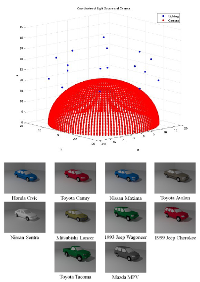
age in classiﬁcation and modeling tasks. One dataset

is a EO Synthetic Vehicle Database, which contains

several different cars, various lighting conditions, and

multiple viewing angles, as shown in Figure 3. This

dataset tests the algorithms ability to model an en-

tire vehicle manifold across these different scenarios.

The other dataset is the Shefﬁeld (previously UMIST)

database, which contains several images of faces with

varying poses. For all datasets, a 13x13 kernel is used

for training and testing the dataset.

Figure 3: EO Synthetic Vehicle Database. The top image

shows the different camera and lighting positions of the

database and the images below show the different vehicles.

3.2 Results 1

The ﬁrst dataset is the EO Synthetic Vehicle database.

The results are shown in Table 2. We used a full 360

view of each vehicle and one lighting condition to

train and test the validity of the technique. Weight ma-

trices were trained with all views and tested accord-

ing to the closest distance between each point (Eu-

clidean distance). It is observed that by concatenating

all of the results from the nonlinear dimensionality

reduction, we are able to keep some of the distinc-

tion found in the orders rather than summing them.

When we start adding more principal components ob-

tained from the the method, we are able to increase

the recognition result. It is observed that the GNLA

architecture and concatenating the orders is able to

decrease the number of principal components while

keeping the recognition result of the vehicles high.

3.3 Results 2

The second dataset we use is the Shefﬁeld database.

The results are shown in Table 3. We split the whole

database into two for testing and training sets. Once

we have trained the network with the training set,

we then perform nonlinear dimensionality reduction

Gaussian Nonlinear Line Attractor for Learning Multidimensional Data

135

Table 1: Training times for each stage of the algorithms.

Runtime Original Current Kernel Kernel (No zeros)

Stage 1 N/A 15.2 min 15.2 min 15.2 min

Stage 2 1280 min 95.3 min 3.35 min 2.4 min

Stage 3 87.5 min 87.5 min 3.08 min 2.21 min

Stage 4 10.8 min 10.8 min 10.8 min 10.8 min

Total Runtime 1378.3 min 208.8 min 32.43 min 30.61 min

Table 2: Recognition results on the EO Synthetic Vehicle Database.

# Prin. Comp. NLA Reg. NLA Concat. GNLA Reg. GNLA Concat.

1 47.50 60.56 35.83 43.89

2 59.72 66.94 82.78 76.94

3 86.67 79.72 63.06 85.28

4 61.39 85.00 76.94 88.61

5 63.89 86.11 81.67 88.89

6 69.17 88.06 85.00 91.11

7 66.94 87.50 86.39 91.39

8 75.28 88.89 87.22 92.22

9 72.22 86.39 91.39 95.00

10 78.61 87.22 91.94 94.72

All 99.19 85.28 99.44 99.17

Table 3: Recognition results on the Shefﬁeld Database.

Algorithm % Recognition

PCA 86.87

KPCA 87.64

LDA 90.87

DPCA 92.90

DCV 91.51

B2DPCA 93.38

GNLA 93.33

GNLA (concat) 94.07

and then found the closest match using Euclidean

distance. We have found that the GNLA architec-

ture works well to recognize the different faces. It

is observed that the GNLA network with concatenat-

ing the orders produced the best results. One of the

major components about the GNLA architecture is

that it runs much faster than the previous architecture.

Run time for one instance of the NLA architecture for

this dataset takes 8.2 hours, while an instance of the

GNLA architecture will take 0.8 hours.

3.4 Discussion

The biggest concern when using associative networks

is that these algorithms work best using orthogonal

data. Given a large dataset that has only small vari-

ances between different classes while having large

variances within the classes, the data is much harder

to classify with the network. Ideally, the network

should have all orthogonal inputs so that modeling

and classiﬁcation of the data are much easier.

With the GNLA architecture, we are able to in-

crease orthogonality by reducing the number of inputs

sent to a given neuron. This is done by only using a

given area for computation of the algorithm. If the

input image is not any of the trained images, we will

see that the image will diverge in the portions of the

data that have the highest variance. Portions of the

image that contain background information will not

be able to converge or diverge since those sections do

not vary.

More importantly, depending on the relationship

created by the NLA architecture for the node connec-

tions, some relationships have a stronger discerning

ability than others, meaning that the nonlinear line

that has been created to model the relationship of the

nodes should have the smallest error (smallest devi-

ation from the created line). For example, if the im-

age wants to converge to one of the trained images,

we must allow those portions with stronger discern-

ing ability to function more than those portions that

are unable to converge or diverge from the input.

Since the NLA architecture allows a summation of

the relationships of the different nodes to estimate one

speciﬁc node, we must allow the portions that have

more discerning ability to be forefront in the weight-

ing scheme. This is why the Gaussian NLA architec-

ture is able to reduce the run times of the algorithm

and increase the convergence rate. Sections of the

object region are assumed to have high amounts of

variability for the relationship created by the NLA in

NCTA 2015 - 7th International Conference on Neural Computation Theory and Applications

136

that speciﬁc area to all have high discerning ability,

thus allowing better convergence of trained images

and better divergence characteristics for untrained im-

ages.

4 CONCLUSIONS

The proposed GNLA architecture using the concate-

nation of the orders and the locality preserving algo-

rithm works well for recognition tasks and for reduc-

ing the amount of computation time. Previous archi-

tectures are much slower and have decent recognition

results, but by incorporating spatial information in the

weighting of the architecture, we are able to increase

the recognition results for a smaller number of dimen-

sions while reducing the computation time. We plan

to improve the weighting performance by exploring

different weighting schemes to weight those portions

of the network that are able to produce signiﬁcant re-

sults.

REFERENCES

Auda, G. and Kamel, M. (1997). Cmnn: cooperative mod-

ular neural networks for pattern recognition. Pattern

Recognition Letters, 18(11):1391–1398.

Golub, G. H. and Reinsch, C. (1970). Singular value de-

composition and least squares solutions. Numerische

Mathematik, 14(5):403–420.

Gomi, H. and Kawato, M. (1993). Recognition of manip-

ulated objects by motor learning with modular archi-

tecture networks. Neural Networks, 6(4):485–497.

Gottumukkal, R. and Asari, V. K. (2004). An improved

face recognition technique based on modular pca ap-

proach. Pattern Recognition Letters, 25(4):429–436.

Guido, W., Spear, P., and Tong, L. (1990). Functional com-

pensation in the lateral suprasylvian visual area fol-

lowing bilateral visual cortex damage in kittens. Ex-

perimental brain research, 83(1):219–224.

Happel, B. L. and Murre, J. M. (1994). Design and evolu-

tion of modular neural network architectures. Neural

networks, 7(6):985–1004.

Hopﬁeld, J. J. (1982). Neural networks and physical sys-

tems with emergent collective computational abili-

ties. Proceedings of the national academy of sciences,

79(8):2554–2558.

Lewis, J. E. and Glass, L. (1991). Steady states, limit

cycles, and chaos in models of complex biological

networks. International Journal of Bifurcation and

Chaos, 1(02):477–483.

Roweis, S. T. and Saul, L. K. (2000). Nonlinear dimension-

ality reduction by locally linear embedding. Science,

290(5500):2323–2326.

Seow, M.-J., Alex, A. T., and Asari, V. K. (2012). Learning

embedded lines of attraction by self organization for

pose and expression invariant face recognition. Opti-

cal Engineering, 51(10):107201–1.

Seow, M.-J. and Asari, V. K. (2004). Recurrent network

as a nonlinear line attractor for skin color association.

In Advances in Neural Networks–ISNN 2004, pages

870–875. Springer.

Seow, M.-J. and Asari, V. K. (2006). Recurrent neural net-

work as a linear attractor for pattern association. Neu-

ral Networks, IEEE Transactions on, 17(1):246–250.

Tononi, G., Sporns, O., and Edelman, G. M. (1999). Mea-

sures of degeneracy and redundancy in biological net-

works. Proceedings of the National Academy of Sci-

ences, 96(6):3257–3262.

Zhang, K. (1996). Representation of spatial orientation

by the intrinsic dynamics of the head-direction cell

ensemble: a theory. The journal of neuroscience,

16(6):2112–2126.

Gaussian Nonlinear Line Attractor for Learning Multidimensional Data

137