Neurosolver Learning to Solve Towers of Hanoi Puzzles
Andrzej Bieszczad and Skyler Kuchar
Computer Science, California State University Channel Islands, One University Drive, Camarillo, CA 93012, U.S.A.
Keywords: Neural Network, Neurosolver, General Problem Solving, Search, State Spaces, Temporal Learning, Neural
Modeling, Towers of Hanoi.
Abstract: Neurosolver is a neuromorphic planner and a general problem solving (GPS) system. To acquire its problem
solving capability, Neurosolver uses a structure similar to the columnar organization of the cortex of the brain
and a notion of place cells. The fundamental idea behind Neurosolver is to model world using a state space
paradigm, and then use the model to solve problems presented as a pair of two states of the world: the current
state and the desired (i.e., goal) state. Alternatively, the current state may be known (e.g., through the use of
sensors), so the problem is fully expressed by stating just the goal state. Mechanically, Neurosolver works as
a memory recollection system in which training samples are given as sequences of states of the subject system.
Neurosolver generates a collection of interconnected nodes (inspired by cortical columns), each of which
represents a single point in the problem state space, with the connections representing state transitions. A
connection map between states is generated during training, and using this learned memory information,
Neurosolver is able to construct a path from its current state, to the goal state for each such pair for which a
transitions is possible at all. In this paper we show that Neurosolver is capable of acquiring from scratch the
complete knowledge necessary to solve any puzzle for a given Towers of Hanoi configuration.
1 INTRODUCTION
The goal of the research that led to the original
introduction of Neurosolver, as reported in
(Bieszczad and Pagurek, 1998), was to design a
neuromorphic device that would be able to solve
problems in the framework of the state space
paradigm. Fundamentally, in this paradigm, a
question is asked how to navigate a system through
its state space so it transitions from the current state
into some desired goal state. The states of a system
are correspond to points in an n-dimensional space
where each dimension is a certain characteristics of
the system. Trajectories in such spaces formed by
state transitions represent behavioral patterns of the
system. A problem is presented in this paradigm as a
pair of two states: the current state and the desired, or
goal, state. If a sensory system is used, then the
problem can be stated by just indicating the desired
state, since the current state is detected by the sensors.
A solution to the problem is a trajectory between the
two points in the state space representing the current
state and the goal state.
Neurosolver can solve such problems by first
building a behavioral model of the subject system and
then by traversing the recorded trajectories during
both searches and resolutions (Bieszczad, 2006;
2007, 2008, 2011). This processes will be described
with more detail in the following sections. The
learning is probabilistic, so in many respects this
approach is similar to Markov Models (Markov,
2006). However, in some cases, any solution is a good
solution, so rather than acquiring a behavioral model
of the subject system, a random process can be used
to detect all possible transitions between any two
states. For example, paths can be constructed in a
maze through allowing an artificial rat driven by a
Neurosolver-based brain to explore the limits of the
maze (e.g., the walls) (Bieszczad, 2007).
In this paper, we demonstrate that Neurosolver
can solve Towers of Hanoi puzzles with three towers.
Conceptually, exactly same approach would be taken
for any number of towers; we discuss that at the end
of the paper. We explore the probabilistic aspects of
the models for this particular application, and observe
that they do not bring significant gains in
functionality, while slowing down the efficiency of
the searches. As could be expected, puzzles with
larger number of disks require significantly more
training steps to explore all valid trajectories in the
state space. Nevertheless, allowing Neurosolver to
explore the state space sufficiently guarantees that the
best solution is found for any puzzle.
28
Bieszczad, A. and Kuchar, S..
Neurosolver Learning to Solve Towers of Hanoi Puzzles.
In Proceedings of the 7th International Joint Conference on Computational Intelligence (IJCCI 2015) - Volume 3: NCTA, pages 28-38
ISBN: 978-989-758-157-1
Copyright
c
2015 by SCITEPRESS – Science and Technology Publications, Lda. All rights reserved
1.1 Inspirations from Neuroscience
The original research on Neurosolver modeling was
inspired by Burnod’s monograph on the workings of
the human brain (Burnod, 1988). The class of systems
that employ state spaces to present and solve
problems has its roots in the early stages of AI
research that derived many ideas from the studies of
human information processing; among them on
General Problem Solver (GPS) (Newell and Simon,
1963). This pioneering work led to very interesting
problem solving (e.g. SOAR (Laird, Newell, and
Rosenbloom, 1987)) and planning systems (e.g.
STRIPS (Nillson, 1980).
Neurosolver employs activity spreading
techniques that have their roots in early work on
semantic networks (e.g., (Collins and Loftus, 1975)
and (Anderson, 1983)).
1.2 Neurosolver
Neurosolver is a network of interconnected nodes.
Each node represents a state in the problem space.
Rather than considering all possible states of the
subject system, Neurosolver generates nodes only for
states that were explicitly used during the training,
although in principle, in future some hardware
platforms could be easier to implement with
provisions for all states rather than creating them on
demand. In its original application, Neurosolver is
presented with a problem by two signals: the goal
associated with the desired state and the sensory
signal associated with the current state. A sequence of
firing nodes that Neurosolver generates represents a
trajectory in the state space. Therefore, a solution to
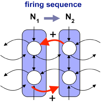
Figure 1: Neurosolver learning rule.
the given problem is a succession of firing nodes
starting with the node corresponding to the current
state of the system, and ending with the node
corresponding to the desired state of the system.The
node used in Neurosolver is based on a biological
cortical column (references to the relevant
neurobiological literature can be found in (Bieszczad
and Pagurek, 1998)). In this simplified model, the
node, an artificial cortical column, consists of two
divisions, the upper and the lower, as illustrated in
Figure 1. The upper division is a unit integrating
internal signals from other upper divisions and from
the control center providing the limbic input (i.e., a
goal or — using a more psychological term — a
drive, or desire, that is believed to have its origins in
the brain’s limbic system). The activity of the upper
division is transmitted to the lower division where it
is subsequently integrated with signals from other
lower divisions and the thalamic input (i.e., the signal
from the sensory system that is relayed through the
brain’s thalamus; for example, a visual system that
recognizes the current configuration of the Towers of
Hanoi puzzle). The upper divisions constitute a
network of units that propagate search activity from
the goal, while the lower divisions constitute a
network of threshold units that integrate search and
sensory signals, and subsequently generate a
sequence of firing nodes; a resolution of the posed
problem (see Figure 2). The output of the lower
division is the output of the whole node.
The function of the network of upper divisions is
to spread the search activity along the intra-cortical
(i.e., upper-to-upper division) connections (as shown
in Figure 3) starting at the original source of activity:
the node associated with the goal state that receives
the limbic input (representing what is desired). This
can be described as a search network because the
activity spreads out in reverse order from that node
along the learned trajectories in hope to find a node
that receives excitatory thalamic input that indicates
that the node corresponds to the current state of the
system. At that node, the activities of the upper and
lower divisions are integrated, and if the combined
activity exceeds the output threshold, the node fires.
The firing node is the trigger of a resolution. The
resolution might be only one of many, but due to the
probabilistic learning it is best in the sense that it was
the most common in the training.
The process of spreading activity in a search tree
is called goal regression (Nillson, 1980). The
implementation on a digital computer is discrete in
that it follows the recalculations of states in cellular
networks. Double-buffering is used to hold the
Neurosolver Learning to Solve Towers of Hanoi Puzzles
29
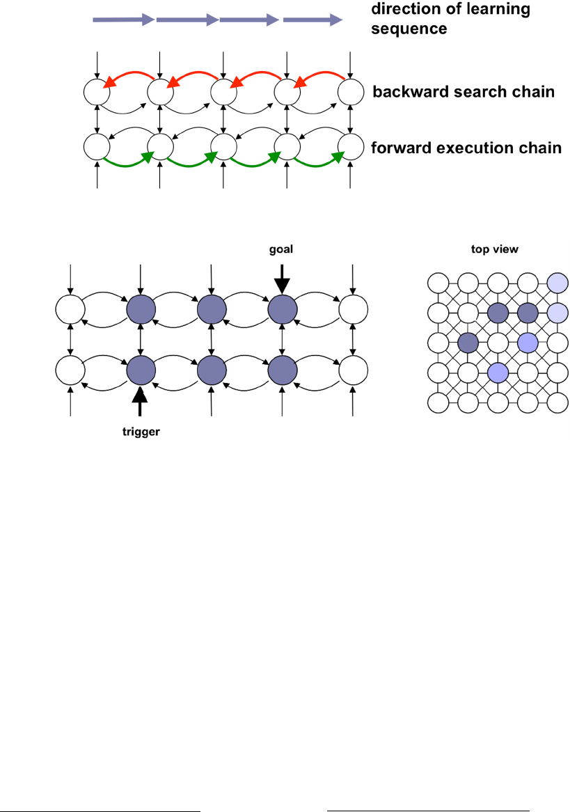
Figure 2: Learning state space trajectories through bi-directional traces between nodes corresponding to transitional states of
the system.
Figure 3: Search in Neurosolver. The externally induced activity is propagated from the node representing the goal state along
the connections between the upper divisions of the nodes in the reverse direction to the direction in which the training samples
were presented. All such pathways are branches in the search tree.
current state of Neurosolver
1
at some time tick t,
while the next state at time tick t+1 is calculated; the
buffers are swapped after that is complete
2
.
The purpose of the network composed of lower
divisions and their connections is to generate a
sequence of output signals from firing nodes (along
the connections shown in Figure 5). Such a sequence
corresponds to a path between the current state and
the goal state, so it can be considered a solution to the
problem. As we said, a firing of the node representing
the current state triggers a solution. Each subsequent
firing node sends action potentials through the
outgoing connections of its lower division. These
signals may cause another node to fire especially if
that node’s attention (i.e., the activity in the upper
division; also called expectation) is sufficiently high,
as that may indicate that the node is part of the search
tree. In a way, the process of selecting the successor
1
It is important not to confuse the states of Neurosolver
with the states of the subject system that Neurosolver is
modeling.
in the resolution path is a form of selecting the node
most susceptible to firing. A firing node is inhibited
for some time afterwards to avoid oscillations. The
length of the inhibition determines the length of
cycles that can be prevented.
Neurosolver exhibits goal-oriented behavior
similar to that introduced in (Deutsch, 1960).
The strength of every inter-nodal connection is
computed as a function of two probabilities: the
probability that a firing source node will generate an
action potential in this particular connection and the
probability that the target node will fire upon
receiving an action potential from the connection (as
shown in Equation 1).
To compute the probabilities, statistics for each
division of the node (both the upper and the lower)
and each connection are collected as illustrated in
Figure 5. The number of transmissions of an action
2
In theory, alternate implementations — for example
utilizing hardware to propagate analog signals — could be
more efficient, but at the moment are hard to realize in
practice.
NCTA 2015 - 7th International Conference on Neural Computation Theory and Applications
30
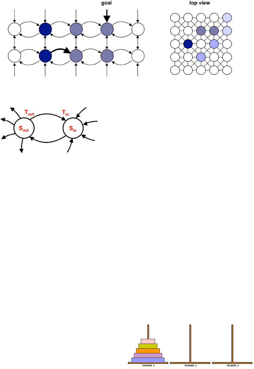
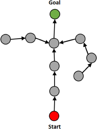
Figure 4: Resolution in Neurosolver. When the search activity integrates with the thalamic input in the node representing the
current state of the system, it triggers a chain reaction of firing nodes towards the node representing the desired — goal —
state, from which the search activity in the upper divisions had originated.
Figure 5: Statistics collected for computation of the
connection strength between nodes.
potential (i.e., transfer of the activity between two
divisions) T
out
is recorded for each connection.
The total number of cases when a division positively
influenced other nodes S
out
is collected for each
division. A positive influence means that an action
potential sent from a division of a firing node to
another node caused that second node to fire in the
following time tick. In addition, statistical data that
relate to incoming signals is also collected. T
in
is the
number of times when an action potential transmitted
over the connection contributed to the firing of the
target node and is collected for each connection. S
in
,
collected for each division, is the total number of
times when any node positively influenced the node.
With such statistical data, we can calculate the
probability that an incoming action potential will
indeed cause the target node to fire. The final formula
that is used for computing the strength of a connection
(shown in Equation 1) is the likelihood that a firing
source node will induce an action potential in the
outgoing connection, multiplied by the likelihood that
the target node will fire due to an incoming signal
from that connection:
P = P
out
P
in
= (T
out
/S
out
) (T
in
/ S
in
) (1)
1.3 Problem: Towers of Hanoi
Towers of Hanoi puzzle is a problem of moving a set
of disks between a pair of pegs (“towers”) utilizing
one or more auxiliary pegs with the rule that a larger
disk can never be placed on top of a smaller disk. A
generalized versions of the problem is to transition
between any two disk configurations observing the
same rules. The former is just a specific version of the
latter, so in this paper we consider the generalized
version of the puzzle.
Commonly, three towers are used in the puzzles;
however, that number can also be generalized. For
example, a puzzle with four towers is called Reve’s
puzzle. While there are known algorithms to find best
solutions to puzzles (i.e., the transition between the
start configuration and the goal configuration with the
minimal disk moves), there is no known algorithm
that can deal with the exponential explosion of
complexity for problems with larger number of disks.
There exists a presumed solution (Stewart, 1941); its
correctness is based on Frame-Stewart conjecture and
has been verified for four towers with up to 30 disks.
In this paper, we deal with puzzles with three
towers. A version with 5 disks is shown in Figure 6.
2 IMPLEMENTATION
Towers of Hanoi puzzle (often also called game) fits
very well into the state space paradigm: each disk
configuration corresponds to a state in the game state
space, and a path between any two points in the state
Figure 6: The Towers of Hanoi puzzle with three towers.
Neurosolver Learning to Solve Towers of Hanoi Puzzles
31
space is a solution to a puzzle for which these two
states are the starting and the goal states. Depending
on the number of disks the state space might be larger
or smaller, but the fit for the paradigm is not affected.
A question then arises if Neurosolver that is
designed to work with problems posed in the terms of
state spaces can indeed be used to tackle Tower of
Hanoi game problems.
2.1 Modeling Towers of Hanoi
In our implementation, each state of the puzzle is
represented as a string as the following examples
show:
•
3 disks: [000,000,123]
•
4 disks: [0012,0003,0004]
•
5 disks: [12345,00000,00000] (see Figure 6)
Here, each tower is represented by n numbers,
separated by a comma where n represents the number
of disks. The example string with 5 disks (n=5)
represents the configuration shown in Figure 4. The
goal state of all disks on peg 3 would be
[00000,00000,12345]. This method of encoding the
state of the game is simple yet also uniquely readable
and convenient as input to Neurosolver. Such
representation could be easily obtained using a
number of methods; for example applying image
processing potentially with some machine learning
techniques for classification. Such preprocessing is
outside of the scope of this paper, so we assume that
the input data are already in this format.
The hypothesis is that after training, Neurosolver
will be able to solve any puzzle problem; i.e., find a
path in the state space of the puzzle going from any
state A, to the goal state B, that can also be any of the
states. Typically the goal is to start with all disks in
tower 1, and move all of them to tower 3; the stated
hypothesis encompasses such a specific case.
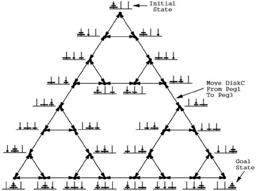
Figure 7 shows a partial state space of a puzzle
with three towers and three discs. Only valid states
and valid transitions are shown in the diagram.
2.2 Modeling Neurosolver
Neurosolver consists of a collection of nodes
representing the configurations of the Tower of Hanoi
game.
Each node has two parts, an upper division, which
contains connections for searching, and a lower
division, which contains connections for actually
solving a problem. The upper level can also be
considered the desire, or goal part of the node,
whereas the lower level represents the current
configuration (as determined by the sensory input) as
well as a controller for forcing disk moves that are
required to get to the goal configuration. Each node
representing a single configuration is connected to
one or more nodes representing other valid
configurations. Neurosolver training is the process of
building nodes corresponding to configurations that
are encountered in the training samples and
constructing a connection map between the nodes.
The connections represent moves of a single disk.
As explained earlier, the connections can have
associated weights that vary based on parameters
such as transitional frequencies, however as we will
see, this does not affect the functional effectiveness
of the model in solving Towers of Hanoi problems.
Figure 7: A partial state space for Towers of Hanoi puzzle with three towers and three discs. Only valid states are included;
i.e., the states that can be reached observing the puzzle rules.
NCTA 2015 - 7th International Conference on Neural Computation Theory and Applications
32
2.3 Neurosolver Operation
Neurosolver requires three main stages to solve a
problem:
• training,
• searching, and
• solving.
2.3.1 Training
Training is responsible for generating state nodes and
for building the connection map between subsequent
states observed in training sequences. This can be
done through various types of training, with a
common approach of Neurosolver exploring actual
transitions between states. For this research, we
implemented two methods of training, user-guided,
and random.
In user-guided training, the system just lets the
user play the game, while it records all moves that the
user makes. While this supervised training is very
effective and can capture user’s experience, it is also
extremely slow (and tedious to the expert player) for
all but the smallest state spaces. While the system will
capture and generalize user’s experience, there will
be no explorations for unknown solutions. There is
also exposure to user mistakes in both entering
invalid configurations and suboptimal resolutions. In
that respect, that approach is similar to building an
expert system through knowledge acquisition from
presumed experts. As with expert systems, the
expertise is captured, but there is no guarantee that
best, or even good, solutions are found; simply, the
experts may not know them.
To get much wider exploration of possible
solutions, perhaps unknown to any users (“experts”),
a random training was implemented. In this mode, in
the spirit of stochastic search methods, random but
still valid moves between puzzle configurations (i.e.,
moves that do not violate the rules of the game) are
generated and input to Neurosolver. It then records all
state transitions as inter-nodal connections.
It should be emphasized again that the training
only creates connections between nodes that
correspond to states that were observed; there are
neither nodes nor connections for states that were
never entered. For example, any invalid state does not
have a representation in Neurosolver. If two states are
theoretically connected, but were not part of any
training sample, then Neurosolver will not use this
theoretical link to solve a problem, as it doesn’t know
of such a connection. Hence, in random mode, it is a
prerogative to allow ample time for space
explorations to capture all possible — and valid —
transitions.
There is a profound functional difference between
the models built with two training techniques: the
former (user-guided) is a probabilistic model that
captures preferred solutions; the latter (random)
builds a connection map, but the statistical
observations need to be ignored as they are also
random.
The models built with both techniques generalize
and optimize solutions by potentially concatenating
parts of other paths into a novel solution. For
example, if a path between [123,000,000] and
[000,123,000], and a path between [000,123,000] and
[000,000,123] are both learned, then the system can
solve a problem [123,000,000]→[000,000,123] in
spite of never seeing such a training sequence.
Essentially, in the random method only singular state
transitions may be used in training.
In both training modes we allow selection of the
number of disks to use in the simulator. In the random
mode of training, the user additionally can select how
many training cycles should be used; in the user-
guided mode the number of training cycles is a
function of user’s tutoring persistence. The program
then returns how many states it managed to find out
of the theoretical total. As we can see in Figure 8, and
as no surprise, the larger the number of possible
states, the more training cycles are required.
This step could be much improved by training in
some controlled manner. The state space of the Tower
of Hanoi problem is fairly well structured, so any
controlled training scheme would give very good
results, but we wanted the process to be completely
unsupervised to explore Neurosolver’s capabilities to
capture the complete knowledge from scratch.
Figure 8 shows the effectiveness of the random
training with 1,000,000 training samples (i.e., single
state transitions).
2.3.2 Searching
After the training is complete, Neurosolver will have
built a connection map between numerous states of
the problem domain. The next step is to apply our
goal (”limbic” or desire) and current/start (“thalamic”
or sensory) inputs to the system. Using past
knowledge from training, the search phase is looking
for a plan that will be used to actually solve the given
problem.
The search mechanism is implemented by
traversing the upper level of the nodes (states) and
their connections. The idea behind the search, is that
our goal is our desire; here, the puzzle configuration
Neurosolver Learning to Solve Towers of Hanoi Puzzles
33
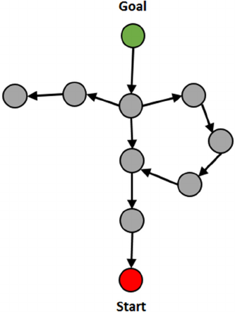
Figure 8: Output capture from Neurosolver shows the
performance of training Neurosolver with 1,000,000
training cycles on a fairly fast iMac (4 GHz Intel Core i7
with 4 cores and 32 GB RAM) using Python 3 with NumPy
version 1.9.2.
The search mechanism is implemented by
traversing the upper level of the nodes (states) and
their connections. The idea behind the search, is that
our goal is our desire; here, the puzzle configuration
that we want. We start from our desired goal state,
and begin to traverse the state space via our learned
connections (see Figure 9).
This is done via an activation value that is applied
to our goal state that is propagated along connections
to the neighboring nodes. Eventually, the hope is that
the spread of the activity will stimulate the node that
also receives the thalamic input to its lower level that
indicates the perceived current state. Once the
activation from the upper level and the lower level are
combined, the node will fire itself from the lower
level, subsequently projecting the activation to its
connected neighboring nodes. If any of the nodes at
the receiving side of these connections has both upper
and lower activation values, then that node will get
increase in the activity sufficient to fire; and so on and
so forth. This constitutes the third stage of
Neurosolver’s operation, the solving. Eventually the
lower level nodes will fire back to the goal. That will
have solved the problem as the goal node gets
inhibited, and consequently the source of the search
activity ceases.
Figure 9: The searching phase of Neurosolver’s operation.
This is a top view of the nodes. Compare with Figure 3 and
Figure 4.
To implement the search stage, a method similar
to cellular automata was used, where at each search
step, the activity of the current node is projected to all
connected nodes, but the activity of those nodes is
recalculated only in the following step (time tick). As
the system progresses through a number of goal
regression cycles, the activity is spread to increasing
number of connected nodes, essentially exploring all
learned paths concurrently in search of the node
associated with the current state.
The benefit of this approach is that it will find the
shortest solution that Neurosolver knows about, as all
possibilities are explored one step at a time. This also
means that any solutions that are close to our current
state will be found quickly.
The downside to this method is that for states that
are far from the goal state, Neurosolver will end up
iterating over many nodes. Depending on the state
space, this could increase dramatically.
One interesting note about searching in the
context of Neurosolver, is that the search is not
actually producing a specific path to the goal. Once
the start node is activated, we do not have a specific
solution. However, the solution is embedded into the
state of Neurosolver itself in the form of activation
values applied to its state nodes. Using this
information, we can construct a path from our start
node back to our goal! The search portion of
Neurosolver produces a directed search tree. Here, as
we traverse backwards through connections in the
upper level of the node, we produce a tree that can be
Disk Count: 1
States found: 3 out of 3 possible.
Runtime: 140.733876 sec
Disk Count: 2
States found: 9 out of 9 possible.
Runtime: 125.792373 sec
Disk Count: 3
States found: 27 out of 27 possible.
Runtime: 126.491495 sec
Disk Count: 4
States found: 81 out of 81 possible.
Runtime: 128.699436 sec
Disk Count: 5
States found: 243 out of 243 possible.
Runtime: 125.649405 sec
Disk Count: 6
States found: 729 out of 729 possible.
Runtime: 128.065042 sec
Disk Count: 7
States found: 2187 out of 2187 possible.
Runtime: 129.181981 sec
Disk Count: 8
States found: 6561 out of 6561 possible.
Runtime: 131.752802 sec
Disk Count: 9
States found: 19683 out of 19683 possible.
Runtime: 135.488318 sec
Disk Count: 10
States found: 48727 out of 59049 possible.
Runtime: 137.897707 sec
NCTA 2015 - 7th International Conference on Neural Computation Theory and Applications
34
used to generate the actual solution from the start
node to the goal node.
Now that we have our first phase complete with a
list of connections, and we have gone through the
searching portion and generated our search tree, we
can move to the final step in solving the problem.
2.3.3 Solving
The last stage of Neurosolver is to use all of the
information collected thus far, and to generate a
solution from the given current state to the specified
goal state.
During the search phase of Neurosolver’s
operation the activity has spread from the goal state
along all possible connections in the upper divisions.
Since the start state has enough activity from both the
upper division (as the result of the search) and lower
division (due to the sensory signal indicating the
current state of the system), it will cause the lower
level to fire, and subsequently excite its neighbor
nodes (along the connections in between the lower
divisions). Since both upper and lower division
activations are required for the lower division to fire,
only the nodes that contain upper division activation
will fire, and that’s only possible for the nodes that
are activated during the search phase. As each lower
division node fires to its neighbor nodes, only the
ones that are activated (i.e., are in an attentive state)
will be activated at levels sufficient to fire; so on and
so forth until the activity reaches the goal state at
which point the problem will have been solved. That
process is illustrated in Figure 10.
Figure 10: The solving phase of Neurosolver’s operation.
As stated earlier, the solving phase still doesn’t
actually give us a complete solution path; it just
causes a sequence of firing nodes. To actually solve
the problem we need to engage the firing of each node
as a trigger for an action that will force the solution
(such as, for example, printing a configuration
associated with the firing node, or, actually
transitioning the puzzle from configuration A to
configuration B in some virtual or real environment).
2.4 Optimizing Neurosolver for Towers
of Hanoi
For this specific application, there is an opportunity
to apply some modifications to the operation that
diverge from the original intent of Neurosolver.
Again, for this particular application owing to the fact
that the connection weights are ignored, we can just
reverse the search path that led from the goal state to
the current state.
There are two optimizations that we performed
during the search phase that yielded a direct solution;
i.e., the shortest path to the goal.
•
First, let’s observe that since the activity of the
lower divisions of the nodes will spread in the
opposite direction to that of the upper divisions
(since we ignore the probabilities). This means
that every branch of the search tree leads to the
goal if traversed in the opposite direction to the
flow of search. This has the implication that there
are no dead ends; essentially, all branches that do
not lead to the goal, or that are loops, are cut out.
It is clearly seen in Figure 10 that shows that the
solving activity (starting in the start/current node)
cannot go “against the traffic” into any of the
branches.
•
The second optimization is that during the search
phase, we only create directed search connections
if the node has not already been activated in the
progression of the current search. This is
essentially “shutting down” the node during the
search after it conducts the search activity first
time. This follows the observation that if during
the search the node we are trying to move to has
already been activated previously, we must be in
a loop, since the search activity must have been
carried over some other path first. Since that other
path evidently carried the activity faster, the path
that is attempted now must be a longer, less
optimal path; hence, no learning should take
place, so no connection is made. This has the
effect of breaking any loops, since the last
connection is a loop is prevented. Since any loop
Neurosolver Learning to Solve Towers of Hanoi Puzzles
35

is prevented, each path is a loop-less branch;
hence, it will be effectively pruned by the effects
of the first optimization.
Using the above two optimizations, the only path
from the current state to the goal state is the shortest
optimal path; the best possible solution.
3 CONCLUSIONS
Neurosolver was able to solve Towers of Hanoi
problems without knowing anything specific about
the problem domain. Figure 11 and Figure 12 show
the results of tests in solving problems in three-tower
puzzles with three and with nine disks respectively.
Substantially longer training was required for
building a model for the nine-disc version. It took
1,000,000 steps vs. 10,000 that were sufficient to
create a model for the four disc version. Evidently,
Neurosolver suffers from the similar problem as other
methods that have been tried to solve Towers of
Hanoi puzzle problems: exponential explosion.
However, by not having all possible states in the
system (as the system is prevented from entering
illegal states), the state space is significantly reduced.
That has a positive effect on the efficiency of
searches. The downside of this is that the training
sessions must be sufficiently long to ensure that all
legal states are included in the training (and hence in
the model), since otherwise some problems may not
be solvable, or their solutions might not be optimal.
The approach taken here considers the shortest
path as the best. That may not necessarily be true. Just
like avoiding bad parts of the city while planning
errands some applications may have the quality of
problem solutions evaluated by another measure. One
aspect of such evaluation might be based on the
frequency of state transitions, so the strength of the
connections that Neurosolver accumulates may be
needed. As we said, it’s an unlikely scenario in the
case of Towers of Hanoi, and accordingly we did not
find much use of that capability.
One observation about using the connection
strengths in searches, was that extremely high values
of initial activation were needed to extend the reach
of the search activity from the goal node to the current
node; the more complex the puzzle (more discs), the
higher initial activity was needed. This is because at
every node, the amount of activation is reduced by a
certain percentage depending on the distribution of
3
This is clearly the area in which an analog implementation
of Neurosolver would be superior. The analog search signal
probabilities amongst the connections. To understand
this, let’s consider the case where all paths are equally
likely, and there are just two outgoing connections
from each node. The “resistance” will be 50% of the
current activation and the projection is split between
the two neighbors. Using this simple observation, we
can see that to move through n consecutive nodes, we
will need an activation value of 2
n
, as each node will
reduce our activation by 2.
Figure 11: The optimal solution to a problem in a three-
tower four-disc Towers of Hanoi puzzle.
Finding the right activation amount is a problem in
itself: too high value might lead to an infinite search,
as all paths will be activated; too low value may not
spread far enough to reach the current node. In both
cases no solution will be generated. Finding the
minimal value sufficient to find a solution requires an
incremental approach in which the activity is
gradually increased, and that unfortunately leads to
increase in the processing as the whole search must
be redone for the new value
3
.
Taking all of these divagations into account, in
the case of this application, we found that ignoring the
connection strengths offered not only the quickest
solutions, but also had the added benefit of
guaranteeing the shortest path; i.e., the optimal
solution for a Towers of Hanoi puzzle.
would be continuously increased until one of the nodes
fires.
States found: 81 out of 81 possible.
Searching...
Start found 15 nodes away, out of 81
states, after checking 80 nodes.
Solving...
1234,0000,0000
0234,0001,0000
0034,0001,0002
0034,0000,0012
0004,0003,0012
0014,0003,0002
0014,0023,0000
0004,0123,0000
0000,0123,0004
0000,0023,0014
0002,0003,0014
0012,0003,0004
0012,0000,0034
0002,0001,0034
0000,0001,0234
0000,0000,1234
Solution Length: 15
Runtime: 0.260015 sec
NCTA 2015 - 7th International Conference on Neural Computation Theory and Applications
36
Figure 12: The optimal solution to a problem in a three-
tower four-disc Towers of Hanoi puzzle. Note that most of
the steps are not shown; only the beginning and the end of
the solution are included.
It was also interesting to observe that the “search”
was simply an encoding of activation data across
Neurosolver itself, without a clear and specific path
being generated. But by using this data, a solution
could be constructed.
For the Tower of Hanoi problem, Neurosolver
worked extremely well. Although this problem did
not take full advantage of Neurosolver capabilities,
through tackling it we did show again that in fact
Neurosolver can solve state-space problems without
having any intrinsic knowledge about the specifics of
the problem domain. That reaffirms our conviction
that Neurosolver indeed is a general problem solver.
4 FUTURE
We are in the process of expanding our experiments
to generalized Towers of Hanoi puzzles like Reve’s
puzzle. In theory, Neurosolver should be able to solve
problems for these puzzles since they also can be
modeled by state spaces.
It is evident that for applications in which
connection strengths are desirable, the issue with
selecting appropriate initial search activity is of
paramount importance. Baring a somewhat elusive
hardware-based analog implementations of
Neurosolver, a good approach could be to set the
activity of each subsequent node to the same activity
at each step of the computation. We are expanding
our model to use activation functions other than the
linear function used in the current implementation
(threshold, sigmoidal, etc.). For this round, we had it
on a back burner, since we did not need to use
probabilities in the experiments with tackling Towers
of Hanoi problems.
While adding front end sensory and back end
effector interfaces would not bring much to the
fundamentals of Neurosolver’s operation, it would
create a more realistic exploratory and demonstration
environment. We are actually applying Neurosolver
in a robot that has a LIDAR scanner as the sensor and
engine-power wheels as the effectors (Bieszczad,
2015). Nevertheless, in the spirit of deep learning we
are also planning to use puzzle images rather than
encoded configurations for training. For that, we will
add an unsupervised configuration classifier as a front
end (e.g., a Support Vector Machine), and use the
classifier’s output as the input to Neurosolver. While
it will necessarily take some time for the classifier to
categorize all puzzle configurations consistently, we
hypothesize that given sufficient time, Neurosolver
will acquire the same level of capabilities as with the
tutoring and random methods. We conjecture that
Neurosolver will need to utilize the probabilities, so
that the inter-nodal connectivity has a chance to
evolve to a stable point after the unavoidable chaos
caused by initial poor input from the classifier.
REFERENCES
Anderson, J. R., 1983. A spreading activation theory of
memory. In Journal of Verbal Learning and Verbal
Behavior, 22, 261-295.
Bieszczad, A. and Pagurek, B., 1998. Neurosolver:
Neuromorphic General Problem Solver. In Information
Sciences: An International Journal 105, pp. 239-277,
Elsevier North-Holland, New York, NY.
Bieszczad, A., 2008. Exploring Neurosolver’s Forecasting
Capabilities. In Proceedings of the 28th International
Symposium on Forecasting, Nice, France, June 22-25.
Bieszczad A., (2011). Predicting NN5 Time Series with
Neurosolver. In Madani, K., Correia, A., Rosa, A., and
Filipe, J. (Eds.), Computational Intelligence: Revised
and Selected Papers of the International Joint
Conference IJCCI 2009 held in Funchal-Madeira,
Portugal, October 2009 (Studies in Computational
Intelligence). Berlin Heidelberg: Springer-Verlag, pp.
277-288.
Bieszczad, A. and Bieszczad, K., (2007) Running Rats with
Neurosolver-based Brains in Mazes. In Journal of
States found: 19683 out of 19683
possible.
Searching...
Start found 511 nodes away, out of
19683 states, after checking 19207
nodes.
Solving...
123456789,000000000,000000000
023456789,000000000,000000001
003456789,000000002,000000001
003456789,000000012,000000000
000456789,000000012,000000003
001456789,000000002,000000003
001456789,000000000,000000023
000456789,000000000,000000123
…
000000023,000000000,001456789
000000003,000000002,001456789
000000003,000000012,000456789
000000000,000000012,003456789
000000001,000000002,003456789
000000001,000000000,023456789
000000000,000000000,123456789
Solution Length: 511
Runtime: 135.752254 sec
Neurosolver Learning to Solve Towers of Hanoi Puzzles
37
Information Technology and Intelligent Computing,
Vol. 1 No. 3.
Bieszczad, A. and Bieszczad, K., (2006). Contextual
Learning in Neurosolver. In Lecture Notes in Computer
Science: Artificial Neural Networks, Springer-Verlag,
Berlin, 2006, pp. 474-484.
Burnod, Y., 1988. An Adaptive Neural Network: The
Cerebral Cortex, Paris, France: Masson.
Collins, Allan M.; Loftus, Elizabeth F., 1975. A Spreading-
Activation Theory of Semantic Processing. In
Psychological Review. Vol 82(6) 407-428.
Deutsch, M., 1960. The Effect of Motivational Orientation
Upon Trust And Suspicion. In Human Relations, 13:
123–139.
Laird, J. E., Newell, A. and Rosenbloom, P. S., 1987.
SOAR: An architecture for General Intelligence. In
Artificial Intelligence, 33: 1--64.
Markov, A. A., 2006. An Example of Statistical
Investigation of the Text Eugene Onegin Concerning
the Connection of Samples in Chains (translation. by
David Link). In Science in Context 19.4: 591-600.
Newell, A. and Simon, H. A., 1963. GPS: A program that
simulates human thought. In Feigenbaum, E. A. and
Feldman, J. (Eds.), Computer and Thought. New York,
NJ: McGrawHill.
Nillson, N. J., 1980. Principles of Artificial Intelligence,
Palo Alto, CA: Tioga Publishing Company.
Russell, Stuart J.; Norvig, Peter (2003), Artificial
Intelligence: A Modern Approach (2nd ed.). Upper
Saddle River, NJ: Prentice Hall, pp. 111-114.
Stewart, B. M. and Frame, J. S., 1941. Solution to Advanced
Problem 3819. In The American Mathematical
Monthly Vol. 48, No. 3 (Mar., 1941), pp. 216-219.
NCTA 2015 - 7th International Conference on Neural Computation Theory and Applications
38
