Choosing Suitable Similarity Measures to Compare Intuitionistic Fuzzy
Sets that Represent Experience-Based Evaluation Sets
Marcelo Loor
1,2
and Guy De Tr
´
e
1
1
Dept. of Telecommunications and Information Processing, Ghent University,
Sint-Pietersnieuwstraat 41, B-9000, Ghent, Belgium
2
Dept. of Electrical and Computer Engineering, ESPOL University,
Campus Gustavo Galindo V., Km. 30.5 Via Perimetral, Guayaquil, Ecuador
Keywords:
Experience-Based Evaluations, Similarity Measures, Intuitionistic Fuzzy Sets.
Abstract:
Which similarity measures can be used to compare two Atanassov’s intuitionistic fuzzy sets (IFSs) that re-
spectively represent two experience-based evaluation sets? To find an answer to this question, several sim-
ilarity measures were tested in comparisons between pairs of IFSs that result from simulations of different
experience-based evaluation processes. In such a simulation, a support vector learning algorithm was used to
learn how a human editor categorizes newswire stories under a specific scenario and, then, the resulting knowl-
edge was used to evaluate the level to which other newswire stories fit into each of the learned categories. This
paper presents our findings about how each of the chosen similarity measures reflected the perceived similarity
among the simulated experience-based evaluation sets.
1 INTRODUCTION
If you ask about comic books suitable for 7-year-old
kids, a coworker who does not like slang expressions
might judge ‘Popeye the Sailor’ as a quite unsuitable
comic book, whereas a coworker who learned eating
spinach due to “they are the source of Popeye’s su-
per strength” might judge it as a totally suitable one.
We deem the evaluations resulting from this kind of
judgments to be experience-based evaluations, which
mainly depend on what each person has experienced
or understood about a particular concept (e.g., ‘comic
books suitable for 7-year-old kids’).
Imagine that your sister is looking for a proper
comic book for your 7-year-old nephew. If you want
to know which of your coworkers could choose a
comic book on behalf of your sister, you might be
interested in measuring the level to which the eval-
uations given by each coworker are similar to your
sister’s evaluations. A problem in such similarity
comparisons is that those experience-based evalua-
tions are fairly subjective and a “pseudo-matching”
between them is possible, i.e., the evaluations could
match even though the evaluators have distinct under-
standings of the evaluated concept (Loor and De Tr
´
e,
2014).
Considering that an experience-based evaluation
could be imprecise and marked by hesitation, in (Loor
and De Tr
´
e, 2014) the authors proposed modeling it
as an element of an intuitionistic fuzzy set, or IFS for
short (Atanassov, 1986; Atanassov, 2012). However,
the authors pointed out that, to compare two IFSs that
represent experience-based evaluation sets, the simi-
larity measures based on a metric distance approach
such as the studied in (Szmidt and Kacprzyk, 2013;
Szmidt, 2014) might not be applicable to the case be-
cause of their implicit assumption about symmetry
and transitivity, which does not reflect judgments of
similarity observed from a psychological perspective
(Tversky, 1977).
To study empirically which of those similarity
measures can be used to compare such IFSs, which is
the main purpose of this paper, we tested those simi-
larity measures in comparisons between pairs of IFSs
resulting from simulations of experience-based eval-
uation processes. Our motivation for this study is to
complement the existing theoretical work within the
context of IFSs to find suitable methods that allow
us to compare experience-based evaluation sets given
from persons that might have different learning expe-
riences.
To simulate an experience-based evaluation pro-
cess, we first made use of a learning algorithm that
uses support vector machines (Vapnik, 1995; Vapnik
Loor M. and De TrÃl’ G.
Choosing Suitable Similarity Measures to Compare Intuitionistic Fuzzy Sets that Represent Experience-Based Evaluation Sets.
DOI: 10.5220/0005600100570068
In Proceedings of the 7th International Joint Conference on Computational Intelligence (ECTA 2015), pages 57-68
ISBN: 978-989-758-157-1
Copyright
c
 2015 by SCITEPRESS – Science and Technology Publications, Lda. All rights reserved
57

and Vapnik, 1998) to learn how a human editor cate-
gorizes newswire stories under a given scenario. We
then made use of the previous knowledge to evalu-
ate the level to which other stories fit into one of the
learned categories and, thus, we obtained the simu-
lated experience-based evaluation sets. Each of the
established learning scenarios included a training col-
lection that contains a certain proportion of opposite
examples in relation to the original data, which con-
sist of manually categorized newswire stories —by
opposite example is meant that, e.g., if a story is as-
signed to a particular category in the original training
collection, the story will not be assigned to the cat-
egory in the training collection related to the current
scenario.
An interesting aspect about testing the similar-
ity measures in that way is that we can observe
how they reflect the perceived similarity between two
experience-based evaluation sets given from dissim-
ilar learning scenarios. For instance, we could test
a similarity measure to observe how it reflects the
perceived similarity between the IFSs given by two
persons who use training collections having examples
that are totally opposite to each other —here, one can
anticipate that the resulting level of similarity will be
the lowest.
The remainder of this work is structured as fol-
lows: Section 2 presents the IFS concept as well as
the similarity measures that were tested; Section 3
describes how the simulated experience-based eval-
uation sets were obtained; Section 4 describes the test
procedure that was carried out for each of the chosen
similarity measures; Section 5 presents the results and
our findings during the testing process; and Section 6
concludes the paper.
2 PRELIMINARIES
This section presents a brief introduction to the IFS
concept and shows how an IFS is used to model
an experience-based evaluation set. Additionally, it
presents some of the existing similarity measures for
IFSs and introduces the formal notation that has been
used throughout the paper.
2.1 IFS Concept
In (Atanassov, 1986; Atanassov, 2012), an intuition-
istic fuzzy set, IFS for short, was proposed as an ex-
tension of a fuzzy set (Zadeh, 1965) and was defined
as follows:
Definition 1 ((Atanassov, 1986; Atanassov, 2012)).
Consider an object x in the universe of discourse X
and a set A ⊆X. An intuitionistic fuzzy set is a collec-
tion
A
∗
= {hx,µ
A
(x),ν
A
(x)i|(x ∈ X)∧
(0 ≤ µ
A
(x) + ν
A
(x) ≤ 1)}, (1)
such that the functions µ
A
: X 7→ [0,1] and ν
A
: X 7→
[0,1] define the degree of membership and the degree
of non-membership of x ∈X to the set A respectively.
In addition, the equation
h
A
(x) = 1 −µ
A
(x) −ν
A
(x) (2)
was proposed in (Atanassov, 1986) to represent the
lack of knowledge (or hesitation) about the member-
ship or non-membership of x to the set A.
2.1.1 Modeling Experience-based Evaluations
An IFS can be used to model an experience-based
evaluation set (Loor and De Tr
´
e, 2014). For in-
stance, X = { ‘Popeye the Sailor’, ‘The Avengers’ }
could represent the ‘comic books’ that you asked your
coworkers to evaluate for, and A could represent a set
of the ‘comic books suitable for 7-year-old kids’. If
so, the IFS A
∗
= {h‘Popeye the Sailor’, 0, 0.8 i,h ‘The
Avengers’, 0.5, 0.3 i} might represent the evaluations
given by one of your coworkers.
2.1.2 IFS Notation
Even though Definition 1 and the previous example
show the difference between the IFS A
∗
and the set
A, as it was suggested in (Atanassov, 1986) we shall
hereafter use A instead of A
∗
as a notation for an IFS.
2.2 Similarity Measures for IFSs
Let A and B be two IFSs in X = {x
1
,···,x
n
}, a sim-
ilarity measure S is usually defined as a mapping
S : X
2
7→ [0,1] such that S(A,B) denotes the level to
which A is similar to B with 0 and 1 representing the
lowest and the highest levels respectively.
Recalling the difference between an IFS P
∗
and
a set P in Definition 1, the IFSs A and B in S(A,B)
correspond to
P
∗
@A
= {hx,µ
P
@A
(x),ν
P
@A
(x)i|(x ∈ X)∧
(0 ≤ µ
P
@A
(x) + ν
P
@A
(x) ≤ 1)},
and
P
∗
@B
= {hx,µ
P
@B
(x),ν
P
@B
(x)i|(x ∈ X)∧
(0 ≤ µ
P
@B
(x) + ν
P
@B
(x) ≤ 1)},
FCTA 2015 - 7th International Conference on Fuzzy Computation Theory and Applications
58

respectively, where P
@A
and P
@B
represent the indi-
vidual understanding of P as seen from the perspec-
tives of the evaluators who provide the IFSs A and B.
This means that, in the context of experience-based
evaluations, S(A, B) measures the similarity between
IFSs A and B with regards to individual understand-
ings of a common set P. For instance, if P represents
a collection of ‘comic books suitable for 7-year-old
kids,’ S(A,B) will measure the similarity between two
experience-based evaluation sets taking into account
the individual understandings of P that the providers
of IFSs A and B might have.
The above clarification is needed because we iden-
tify two approaches in the formulation of similarity
measures for IFSs: a symmetric (or metric distance)
approach, which considers that S(A,B) = S(B,A) al-
ways holds; and a directional approach, which con-
siders that S(A,B) = S(B, A) only holds in situations
in which the evaluators who provide the IFSs A and
B have the same understandings of the common set
behind these IFSs.
2.2.1 Symmetric Similarity Measures
Among others, the following symmetric similarity
measures for IFSs have been studied:
S
H3D
(A,B) = 1 −
1
2n
n
∑
i=1
(|µ
A
(x
i
) −µ
B
(x
i
)|
+ |ν
A
(x
i
) −ν
B
(x
i
)|
+ |h
A
(x
i
) −h
B
(x
i
)|) (3)
and
S
H2D
(A,B) = 1 −
1
2n
n
∑
i=1
(|µ
A
(x
i
) −µ
B
(x
i
)|
+ |ν
A
(x
i
) −ν
B
(x
i
)|), (4)
which are based on Hamming distance (Szmidt and
Kacprzyk, 2000);
S
E3D
(A,B) = 1 −
1
2n
n
∑
i=1

(µ
A
(x
i
) −µ
B
(x
i
))
2
+ (ν
A
(x
i
) −ν
B
(x
i
))
2
+ (h
A
(x
i
) −h
B
(x
i
))
2


1
2
(5)
and
S
E2D
(A,B) = 1 −
1
2n
n
∑
i=1

(µ
A
(x
i
) −µ
B
(x
i
))
2
+ (ν
A
(x
i
) −ν
B
(x
i
))
2


1
2
, (6)
which are based on Euclidean distance (Szmidt and
Kacprzyk, 2000); and
S
COS
(A,B) =
1
n
n
∑
i=1
(µ
A
(x
i
)µ
B
(x
i
) + ν
A
(x
i
)ν
B
(x
i
)
+ h
A
(x
i
)h
B
(x
i
))/

µ
A
(x
i
)
2
+ ν
A
(x
i
)
2
+ h
A
(x
i
)
2

1
2

µ
B
(x
i
)
2
+ ν
B
(x
i
)
2
+ h
B
(x
i
)
2

1
2
, (7)
which is based on Bhattacharyas’s distance (Szmidt
and Kacprzyk, 2013).
2.2.2 Directional Similarity Measures
The following two directional similarity measures for
IFSs have been studied:
S
α
(A,B) = 1 −
1
n
n
∑
i=1
|di f
α
(a
i
,b
i
)|, (8)
where α ∈ [0,1] is called hesitation splitter,
a
i
=

µ
A
(x
i
) + αh
A
(x
i
)
ν
A
(x
i
) + (1 −α)h
A
(x
i
)

and
b
i
=

µ
B
(x
i
) + απ
B
(x
i
)
ν
B
(x
i
) + (1 −α)π
B
(x
i
)

are vector interpretations of the IFS-elements in IFSs
A and B related to x
i
(Loor and De Tr
´
e, 2014), and
di f
α
(a
i
,b
i
) = (µ
A
(x
i
) −µ
B
(x
i
))
+ α(h
A
(x
i
) −h
B
(x
i
)) (9)
is the spot difference between the IFS-elements cor-
responding to x
i
in A and B respectively (Loor and
De Tr
´
e, 2014); and
S
α
@A
(A,B) = ∆
@A
·S
α
(A,B), (10)
which is an extension of (8) based on the weight
∆
@A
∈[0, 1] of a connotation-differential print (CDP)
between A and B as seen from the perspective of the
evaluator who provides A (Loor and De Tr
´
e, 2014).
A CDP is defined as a sequence that represents any
difference in the understandings of the common set
behind IFSs A and B (Loor and De Tr
´
e, 2014). Since
such a difference in understandings is deemed to be
subjective, the assembling of a CDP will depend on
either the perspective of who provides A or the per-
spective of who provides B (i.e., it is directional); so
will do its weight (Loor and De Tr
´
e, 2014).
Choosing Suitable Similarity Measures to Compare Intuitionistic Fuzzy Sets that Represent Experience-Based Evaluation Sets
59

3 SIMULATION
As was mentioned in the introduction, the aim of this
work is to study empirically which of the similar-
ity measures presented in Section 2.2 can be used
to compare experience-based evaluation sets repre-
sented by IFSs. Hence, in this section we describe
both the learning and the evaluation processes that
were used to obtain the IFSs that represent the sim-
ulated experience-based evaluation sets.
3.1 Learning Process
In this part we describe the data, scenarios and algo-
rithm that were employed to simulate how a human
editor categorizes newswire stories.
3.1.1 Learning Data
We made use of the Reuters Corpora Volume I
(RCV1) (Rose et al., 2002), which is a collection of
manually categorized newswire stories provided by
Reuters, Ltd. Specifically, we made use of the cor-
rected version RCV1.v2, which is available (and fully
described) in (Lewis et al., 2004). This collection
has 804414 newswire stories, each assigned to one or
more (sub) categories within three main categories:
Topics, Regions and Industries.
We made use of the 23149 newswire stories in the
training file lyrl2004 tokens train.dat to learn how
to categorize newswire stories into one or more of
the following categories from Topics: ECAT, E11,
E12, GSCI, GSPO, GTOUR, GVIO, CCAT, C12, C13,
GCAT, G15, GDEF, GDIP, GDIS, GENT, GENV,
GFAS, GHEA and GJOB. The interested reader is re-
ferred to (Lewis et al., 2004) for a full description of
these categories.
3.1.2 Learning Scenarios
We established the following scenarios to learn how
to categorize newswire stories into each of the chosen
categories:
- R0: All the stories in the training data preserve the
assignation of the training category in its original
state.
- R20, R40, R60, R80, R100: The assignation of the
training category is opposite to its original state in
the 20%, 40%, 60%, 80% and 100% of the sto-
ries in the training data respectively. The assigna-
tion of the training category in the remainder of
the stories is preserved. The selection of the sto-
ries that do not preserve the original state is made
through a simple random sampling.
For instance, consider the story with code 2286,
which was assigned to the category ECAT. In the sce-
nario R20, if the training category is ECAT and the
story is selected to change its category, the story will
be considered as a nonmember of ECAT.
3.1.3 Learning Algorithm
We made use of an algorithm based on support vec-
tor machines, or SVM for short (Vapnik, 1995; Vap-
nik and Vapnik, 1998), which have been successfully
used in statistical learning theory. Specifically, we
made use of the application of SVMs for the text cat-
egorization problem proposed in (Joachims, 1998),
which has demonstrated superior results to deal with
such a problem (Lewis et al., 2004).
In the context of the text categorization problem,
the words in a newswire story are the features that
determine whether the story belongs or not to a cate-
gory. This follows an intuition in which, according to
his/her experience, a person focuses on the words in a
document to decide whether it fits or not into a given
category.
To use the SVM algorithm, each story must be
modeled as a vector whose components are the words
in the story. A story might contain words such as
‘the’, ‘of’ or ‘at’ that have a negligible impact on
the categorization decision, or words such as ‘learn-
ing’, ‘learned’ or ‘learn’ that have a common stem.
To simplify the vector representation, such words are
usually filtered out and stemmed by using different
algorithms. Hence, for the sake of reproducibility of
the simulation, we made use of the stories in the train-
ing file lyrl2004 tokens train.dat (Lewis et al., 2004),
which already have reduced and stemmed words. For
example, the story with code 2320 has the following
words: tuesday, stock, york, seat, seat, nys, level, mil-
lion, million, million, sold, sold, current, off, exchang,
exchang, exchang, bid, prev, sale, mln.
Since the impact of the words on the categoriza-
tion decision could be different, a weight should be
assigned to each word. Thus, to compute the (ini-
tial) weight of a word in a story (or document), as it
was suggested in (Lewis et al., 2004), we applied the
equation
weight( f ,x) = (1 + lnn( f ,x))ln(|X
0
|/n( f ,X
0
)),
(11)
which is a kind of tf-idf weighting given in (Buckley
et al., 1994) where X
0
is the training collection (i.e.,
the collection of stories in lyrl2004 tokens train.dat),
x ∈ X
0
is a story, f is a word in x, n( f ,x) is the num-
ber of occurrences of f in x, n( f ,X
0
) is the num-
ber of stories in X
0
that contain f , and |X
0
| is the
number of stories in X
0
(i.e., |X
0
| = 23149). For ex-
FCTA 2015 - 7th International Conference on Fuzzy Computation Theory and Applications
60

H
−
H H
+
w
m
b
d
+
d
−
Figure 1: Idea behind the SVM algorithm.
ample, the weight of the word exchang in the story
with code 2320 is given by weight(exchang,2320) =
(1 + ln3) ln(23149/2485) = 4.6834.
After computing the weight of each word in a
story with code i, say x
i
, we represented x
i
as a vector
x
i
= β
i,1
ˆ
f
1
+ ···+ β
i,|F|
ˆ
f
|F|
such that:
- F is a dictionary having all the distinct words in
the training collection X
0
;
- |F| is the number of words in F (for the chosen
training collection, |F| = 47152);
-
ˆ
f
k
is a unit vector that represents an axis related
to a word f
k
∈ F (i.e.,
ˆ
f
k
belongs to a multi-
dimensional feature space in which each dimen-
sion corresponds to a word f
k
∈ F); and
- β
i,k
= weight( f
k
,x
i
) is the weight of f
k
in x
i
(if f
k
is not present in the story, β
i,k
will be fixed to 0).
Since the stories may have different number of words,
each β
i,k
in x
i
was divided by kx
i
k =
√
x
i
·x
i
, i.e., x
i
was transformed to a unit vector (Lewis et al., 2004).
Idea behind the SVM algorithm: So far we have
described how each story x
i
in the training collection
X
0
was represented by a vector x
i
. To describe how
we made use of those vectors (and the resulting ones
later on), in what follows we briefly explain the idea
behind the SVM algorithm (see (Burges, 1998) for a
tutorial about SVM).
In Figure 1 the vectors corresponding to stories
that fit into a given category (i.e., positive examples)
are depicted with gray-circle heads, while the vectors
that do not fit into the category (i.e., negative exam-
ples) are depicted with black-circle heads. The hy-
perplane H separates the positive from the negative
examples —here H is defined by w ·x + b = 0, where
w is a vector perpendicular to H, x is a point lying on
H, and b is the perpendicular distance between H and
the origin. The hyperplane H
+
is parallel to H and
contains the closest positive example to it. The hyper-
plane H
−
is also parallel to H and contains the closest
negative example to it. The margin m = d
+
+ d
−
be-
tween H
+
and H
−
is the largest. The support vectors
are the vectors whose heads lay either on H
−
or H
+
.
To find the hyperplane H that maximizes the mar-
gin between H
+
and H
−
the following quadratic pro-
gramming problem should be solved
Λ =
n
∑
i=1
λ
i
−
1
2
n
∑
i=1, j=1
λ
i
λ
j
y
i
y
j
x
i
·x
j
, (12)
where x
i
and x
j
are the vectors corresponding to
stories in the training collection, y
i
(or y
j
) denotes
whether the x
i
(or x
j
) fits (y
i
= 1) or not (y
i
= −1)
into the category, λ
i
,λ
j
≥ 0, and n is the number of
stories in the training collection. The solution is given
by both
w =
n
∑
k=1
λ
k
y
k
x
k
(13)
and
b = y
k
−w ·x
k
, (14)
for any x
k
such that λ
k
> 0.
To compute both (13) and (14), we made use of the
package SVMLight Version V6.02 (Joachims, 1999).
We issued the command “svm learn.exe -c 1 svm-
TrainingFile svmModelFile”, where svmTrainingFile
is an input file that contains the training vectors for
a category under a given scenario, and svmModelFile
is an output file that contains the solution (or model)
of the scenario-category learning process. Using the
6 scenarios and 20 categories described above, we
obtained 120 scenario-category models during this
learning process —hereafter a model will be referred
to using the nomenclature scenario-category.
3.2 Evaluation Process
Consider a collection of newswire stories X. To eval-
uate the level to which a newswire story x ∈ X fits
into a category, say ECAT, under a given scenario,
say R20, we use the R20-ECAT model, which rep-
resents the experience (or knowledge) acquired after
the previous learning process. After evaluating all the
newswire stories in X, we obtain an evaluation set
for X. This evaluation set corresponds to the simu-
lated experience-based evaluation set given by a per-
son who learned the concept ECAT using the training
data specified in the scenario R20.
The data and the process that were utilized to gen-
erate such simulated experience-based evaluation sets
are described below.
3.2.1 Evaluation Data
We made use of the first 12500 newswire stories in
each of the following files from RCV1.v2 (Lewis
et al., 2004):
- lyrl2004 tokens test pt0.dat,
Choosing Suitable Similarity Measures to Compare Intuitionistic Fuzzy Sets that Represent Experience-Based Evaluation Sets
61

- lyrl2004 tokens test pt1.dat,
- lyrl2004 tokens test pt2.dat and
- lyrl2004 tokens test pt3.dat.
With these 50000 stories, we built 1000 50-story col-
lections.
3.2.2 Obtaining an IFS as a Result of an
Evaluation Process
Let X
k
be one of the 50-story collections that consti-
tute the evaluation data. To evaluate the level to which
a story x
i
∈X
k
fits into a category, say C, under a given
(learning) scenario, say LS, we made use of the LS-C
model resulting from the previous learning process to
obtain an IFS-element hx
i
,µ
C
(x
i
),ν
C
(x
i
)i as follows.
First, we represented x
i
as a vector x
i
= β
i,1
ˆ
f
1
+
··· + β
i,|F|
ˆ
f
|F|
according to the procedure described
in the previous section, where X
0
corresponds to the
training collection in the scenario S.
Then, we made use of w = ω
1
ˆ
f
1
+ ···+ ω
|F|
ˆ
f
|F|
and b in the S-C model to figure out µ
C
(x
i
) and ν
C
(x
i
)
by means of the equations
µ
C
(x
i
) = ˇµ
C
(x
i
)/σ (15)
and
ν
C
(x
i
) =
ˇ
ν
C
(x
i
)/σ (16)
respectively, where
ˇµ
C
(x
i
) =










∑
|F|
j=1
β
i, j
ω
j

+
|
b
|
k
x
i
k
kwk
: (β
i, j
ω
j
> 0) ∧(b < 0);
∑
|F|
j=1
β
i, j
ω
j
k
x
i
k
kwk
: (β
i, j
ω
j
> 0) ∧(b ≥ 0);
0 : otherwise;
(17)
ˇ
ν
C
(x
i
) =










∑
|F|
j=1
|β
i, j
ω
j
|

+b
k
x
i
k
kwk
: (β
i, j
ω
j
< 0) ∧(b > 0)
∑
|F|
j=1
|β
i, j
ω
j
|
k
x
i
k
kwk
: (β
i, j
ω
j
< 0) ∧(b ≤ 0);
0 : otherwise;
(18)
and
σ = max(1, ˇµ
C
(x
i
) +
ˇ
ν
C
(x
i
)),∀x
i
∈ X
k
. (19)
Finally, after computing all the IFS-elements for
each x
i
∈ X
k
, we obtained an IFS that represents the
simulated experience-based evaluations for the stories
in X
k
according to what was learned (or experienced)
about the category C under the scenario LS.
Since we built 1000 50-story collections, we ob-
tained 1000 IFSs for each scenario-category model.
We made use of the notation C
@LS
(X
k
) to denote an
IFS that represents the simulated experience-based
evaluations for the stories in X
k
according to what was
learned about category C under a scenario LS. For
Table 1: IFSs that represent the simulated experience-based
evaluations for the stories in each X
k
∈ {X
1
,··· ,X
1000
} ac-
cording to what was learned about category E11 under the
scenarios R0, R20, R40, R60 and R100 respectively.
E11 X
1
··· X
1000
R0 E11
@R0
(X
1
) ··· E11
@R0
(X
1000
)
R20 E11
@R20
(X
1
) ··· E11
@R20
(X
1000
)
R40 E11
@R40
(X
1
) ··· E11
@R40
(X
1000
)
R60 E11
@R60
(X
1
) ··· E11
@R60
(X
1000
)
R80 E11
@R80
(X
1
) ··· E11
@R80
(X
1000
)
R100 E11
@R100
(X
1
) ··· E11
@R100
(X
1000
)
example, Table 1 shows the IFSs that represent the
simulated experience-based evaluations for the stories
in each X
k
∈ {X
1
,···,X
1000
} according to what was
learned about category E11 under the scenarios R0,
R20, R40, R60 and R100 respectively.
Considering that we chose 20 categories and built
6 scenarios during the learning phase, we obtained a
total of 120000 IFSs during this phase.
4 TESTING
In this section we describe how the similarly measures
presented in Section 2.2 were tested with the IFSs that
represent simulated experience-based evaluation sets.
4.1 A point of Reference for the
Perceived Similarity
Consider a scenario-category model LS-C represented
by both w and b according to the equations (13) and
(14) respectively (see Section 3.1.3). Consider then
a story x
i
∈ X
k
represented by x
i
, where X
k
is one
of the 50-story collections in the evaluation data (see
Section 3.2.2). Consider finally a collection Y
k
=
{y
i
|(y
i
= w ·x
i
+ b)} such that y
i
is the SVM-based
evaluation of story x
i
∈ X
k
fitting into the category
C under the scenario LS. In this context, the decision
about the fittingness of the story x
i
into the category C
under the scenario LS will depend on y
i
: when y
i
> 0,
the decision will be “x
i
fits into C;” when y
i
< 0, the
decision will be “x
i
does not fit into C;” and when
y
i
= 0, no decision will be taken. A visual interpreta-
tion of this decision process is observable in Figure 1:
when y
i
> 0 the head of the vector x
i
corresponding
to story x
i
will be on the H
+
-side, i.e., it will have a
gray-circle head; when y
i
< 0 the head of x
i
will be on
the H
−
-side, i.e., it will have a black-circle head; and
when y
i
= 0 the head of x
i
will be on H (see (Lewis
et al., 2004) for more details about the influence of
this decision process in the text categorization prob-
lem).
FCTA 2015 - 7th International Conference on Fuzzy Computation Theory and Applications
62

Now consider the collections Y
k@L1
and Y
k@L2
having SVM-based evaluations under scenarios L1
and L2 respectively. Consider also y
i@L1
∈Y
k@L1
and
y
i@L2
∈Y
k@L2
. In this situation, when
((y
i@L1
< 0 ∧y
i@L2
< 0)
∨(y
i@L1
> 0 ∧y
i@L2
> 0)
∨ (y
i@L1
= 0 ∧y
i@L2
= 0))
is true, an agreement on decision about the fittingness
of story x
i
between the evaluations given under sce-
narios L1 and L2 occurs.
We made use of the agreements on decisions be-
tween Y
k@L1
and Y
k@L2
to obtain an agreement-on-
decision ratio, AoD for short, which is expressed by
AoD(Y
k@L1
,Y
k@L2
) = n/N, (20)
where n represents the number of agreements on de-
cision between Y
k@L1
and Y
k@L2
, and N represents the
number of stories in X
k
. Since the AoD ratio denotes
how similar the decisions are, we deemed it to be an
indicator of the perceived similarity between the eval-
uations given by two persons that learned (or experi-
enced) C under L1 and L2 respectively.
4.2 Testing Procedure and Settings
As was mentioned in the Introduction, an experience-
based evaluation mainly depends on what an evalua-
tor has experienced or learned about a particular con-
cept. Thus, one could expect that the level of similar-
ity between the evaluation sets given by two evalua-
tors who learned a concept under the same (learning)
scenario will be greater than or equal to the level of
similarity between the evaluation sets given by two
evaluators who learned the same concept under dif-
ferent scenarios. For instance, consider three evalua-
tors: P, Q and R. While P and Q learned about cat-
egory E11 under the same scenario R0, R learned so
under the scenario R80. Consider also that the IFSs
E11
P
@R0
(X
k
), E11
Q
@R0
(X
k
) and E11
R
@R80
(X
k
) repre-
sent the experience-based evaluation sets about the
fittingness of the stories in the 50-story collection
X
k
into category E11 given by P, Q and R respec-
tively. In this context, one could expect that the sim-
ilarity between E11
P
@R0
(X
k
) and E11
Q
@R0
(X
k
) will be
greater than the similarity between E11
P
@R0
(X
k
) and
E11
R
@R0
(X
k
).
We made use of the intuition given above to test
the similarity measures presented in Section 3.2.2.
Since we chose the AoD ratio as an indicator of the
perceived similarity, we first tested it to observe how
the agreement on decisions between two SVM-based
evaluation sets is affected according to their respec-
tive learning scenarios. We then tested the similarity
measures, some of them with different configurations.
4.2.1 Testing the Agreement-on-decision Ratio
Again, one could expect that the AoD ratio between
two SVM-based evaluation sets resulting from the
same scenario will be greater than the AoD ratio be-
tween two SVM-based evaluation sets resulting from
distinct scenarios. Thus, we considered the ques-
tion: is there sufficient evidence in the evaluation data
to suggest that the mean AoD ratio is different af-
ter altering a given percentage of the training data?
To answer this, for each category and for each 50-
story collection, we obtained the AoD ratio between
the SVM-based evaluation set given under scenario
R0 (i.e., R0 is a referent scenario) and each of the
SVM-based evaluation sets given under the scenarios
R0,R20,R40, R60,R80 and R100 respectively. Algo-
rithm 1 shows the steps to obtain the AoD ratios.
Algorithm 1 : Obtaining AoD ratios.
Require: ChosenCategories {see Section 3.1.1}
Require: LearningScenarios {see Section 3.1.2}
Require: 50storyCollections {see Section 3.2.1}
Require: SV MEvals {see Section 4.1}
1: Z ←
/
0 {resulting ratios}
2: for all C ∈ChosenCategories do
3: for all X
k
∈ 50storyCollections do
4: Y
k@R0
← SV MEvals[X
k
][R0][C]
5: for all LS ∈ LearningScenarios do
6: Y
k@LS
← SV MEvals[X
k
][LS][C]
7: r ← AoD(Y
k@R0
,Y
k@LS
)
8: Z[C][LS][X
k
] ← r
9: end for
10: end for
11: end for
12: return Z
4.2.2 Testing the Similarity Measures
First, we applied the following labels and settings to
the similarity measures:
- for (3) and (4), H3D and H2D respectively;
- for (5) and (6), E3D and E2D respectively;
- for (7), COS;
- for (8), VB-α, with α = 0, 1;
- for (10), XVB-α-w, with α = 0,0.5,1 and ∆
@A
=
weightCDP(A,B, w), with w = 0.05,0.1,0.2 as
explained below.
To compute ∆
@A
in the settings of (10), we made use
of weightCDP(A,B,w), where A and B are the IFSs in
the comparison, and w ∈ [0,1] is a value that allows
us to obtain a CDP (see Section 3.2.2) between A and
Choosing Suitable Similarity Measures to Compare Intuitionistic Fuzzy Sets that Represent Experience-Based Evaluation Sets
63

0
+δ
−δ
k = 5
k = 5
cd p
H
cd p
L
Figure 2: Obtaining a CDP and its weight. The bars rep-
resent the spot differences between the elements of IFSs A
and B. The CDPs for the k-highest and the k-lowest IFS-
elements according to A’s perspective are denoted by cdp
H
and cd p
L
respectively.
B according to the wide of the average gap between
the membership and non-membership values as seen
from the perspective of who provides A. The method
weightCDP involves the following steps:
1. Obtain δ ∈ [0, 1] for IFS A by means of
δ =
w
n
n
∑
i=1
(µ
A
(x
i
) + ν
A
(x
i
)). (21)
2. Compute the spot differences among the IFS-
elements in A and B using (9).
3. Order the IFS-elements in A by descending mem-
bership values and then by ascending non-mem-
bership values.
4. Fix k = 0.1n (i.e., k = 5) and obtain the connota-
tion-differential markers (i.e., |,

| and

| (Loor and
De Tr
´
e, 2014)) for the k-highest and the k-lowest
IFS-elements in the arranged IFS A (see Figure 2).
For a spot difference s, the marker will be: | when
|s| ≤ δ;

| when s > δ; and

| when s < −δ.
5. Build the CDPs cd p
H
and cd p
L
with the markers
corresponding to k-highest and the k-lowest IFS-
elements respectively (see Figure 2).
6. Fix w[|] = 1, w[

|] = 0.01 and w[

|] = 0.01, and
compute ∆
@A
by means of
∆
@A
= max
1
k
∑
m∈cd p
H
w[m],
1
k
∑
m∈cd p
L
w[m]
!
(22)
Then, as was done with the agreement-on-deci-
sion ratio, for each category and for each 50-story
collection we obtained the level of similarity between
the IFS given under scenario R0 and each of the IFSs
given under the scenarios R0, R20,R40,R60,R80 and
R100 respectively by means of each of the established
similarity measures. Algorithm 2 shows the steps to
obtain the levels of similarity.
Algorithm 2 : Testing similarity measures.
Require: SimMeasures {see Sections 2.2 and 4.2.2}
Require: ChosenCategories {see Section 3.1.1}
Require: LearningScenarios {see Section 3.1.2}
Require: 50storyCollections {see Section 3.2.1}
Require: IFSEvals {see Section 3.2.2}
1: Z ←
/
0 {resulting levels}
2: for all C ∈ChosenCategories do
3: for all X
k
∈ 50storyCollections do
4: C
@R0
(X
k
) ← IFSEvals[X
k
][R0][C]
5: for all LS ∈ LearningScenarios do
6: C
@LS
(X
k
) ← IFSEvals[X
k
][LS][C]
7: for all S ∈ SimMeasures do
8: l ← S(C
@R0
(X
k
),C
@LS
(X
k
))
9: Z[C][LS][X
k
][S] ← l
10: end for
11: end for
12: end for
13: end for
14: return Z
5 RESULTS AND DISCUSSION
This section presents the results after following the
test conditions described in the previous section.
5.1 Agreement-on-decision Ratio as an
Indicator of the Perceived Similarity
To answer the question is there sufficient evidence in
the evaluation data to suggest that the mean AoD ra-
tio is different after altering a given percentage of the
training data?, we first made use of the collection re-
sulting of Algorithm 1 to compute the averages of the
AoD ratios per scenario-category. We then ran the t-
test for the null hypothesis “the average of the AoD
ratio is the same after altering the r% of the training
data” in contrast to the alternative one “the average of
the AoD ratio is different after altering the r% of the
training data” according to r given in each scenario
(see Table 2).
The results in Table 2 show that, for the scenarios
R20, R40, R60 and R100, the t-values were statisti-
cally significant (p < 0.05). Consequently, we can
say that there is sufficient evidence in the evaluation
data to suggest that the average of the AoD ratio is
different after altering the 20%, 40%, 60% or 100%
of the training data.
Recalling that we deemed the AoD ratio to be an
indicator of the perceived similarity, we can confi-
dently expect that it will be affected by the different
learning scenarios established in the simulation. This
FCTA 2015 - 7th International Conference on Fuzzy Computation Theory and Applications
64

Table 2: Averages of the AoD ratios per scenario-category,
and t-test for the null hypothesis “the average of the AoD
ratio is the same after altering the r% of the training data”
according to r given in each scenario (e.g., r = 20 in sce-
nario R20), where R0 (r = 0) is the referent scenario.
Category R20 R40 R60 R80 R100
C12 0.7292 0.5900 0.4757 0.2897 0.0001
C13 0.7385 0.6091 0.4281 0.2766 0.0002
CCAT 0.9372 0.7505 0.2711 0.0663 0.0001
E11 0.6431 0.5740 0.4722 0.3519 0.0003
E12 0.7156 0.5792 0.4796 0.3080 0.0001
ECAT 0.8187 0.6273 0.4052 0.1853 0.0002
G15 0.7186 0.5954 0.4781 0.3039 0.0002
GCAT 0.9314 0.7472 0.2690 0.0661 0
GDEF 0.6515 0.5717 0.4668 0.3602 0.0002
GDIP 0.7433 0.5990 0.4587 0.2672 0.0002
GDIS 0.7229 0.5951 0.4729 0.3022 0.0002
GENT 0.7066 0.5796 0.4802 0.3209 0.0002
GENV 0.6941 0.6009 0.4812 0.3248 0.0004
GFAS 0.6763 0.5787 0.4882 0.3457 0.0002
GHEA 0.7016 0.5850 0.4636 0.3451 0.0003
GJOB 0.7359 0.5883 0.4542 0.2886 0.0003
GSCI 0.6899 0.5854 0.4844 0.3424 0.0004
GSPO 0.8208 0.6508 0.4130 0.1962 0
GTOUR 0.5383 0.5197 0.4866 0.4663 0.0005
GVIO 0.7551 0.6368 0.4749 0.2796 0.0002
Mean 0.7334 0.6082 0.4452 0.2844 0.0002
stdDev 0.0913 0.0551 0.0643 0.0951 0.0001
N 20 20 20 20 20
df 19 19 19 19 19
t-value 13.06 31.80 38.59 33.67 34025.85
p-value 0 0 0 0 0
0
0.2
0.4
0.6
0.8
1
0 0.2 0.4 0.6 0.8 1
AoD
Linear (AoD)
opposites (%)
perceived similarity
y = −0.9299x + 0.9768
R
2
= 0.9488
Figure 3: Bivariate plot between the averages of the AoD
ratios and the percentage of opposites included in the learn-
ing scenarios. The relationship is represented by means of a
linear model and described by the statistic R (Pearson Prod-
uct Moment Correlation).
can be observed in the bivariate plot depicted in Fig-
ure 3, which shows a strongly negative (or inverse) re-
lationship (R = −0.9741) between the averages of the
AoD ratios and the percentage of opposites included
in the learning scenarios.
5.2 How Each Similarity Measure
Reflects the Perceived Similarity
To observe how each of the configurations of similar-
ity measures given in Section 4.2.2 reflects the per-
ceived similarity between the simulated IFSs, we first
made use of the collection resulting of Algorithm 2
to compute the averages of the levels of similarity per
scenario-category. Then, we obtained linear models
for the relationships between each one of those av-
erages and the percentage of opposites considered in
each scenario. After that, each of the resulting mod-
els was contrasted with the linear model correspond-
ing to the AoD ratio. As an indicator of how well
a similarity measure reflects the perceived similarity,
we computed a manifest index, which is defined by
m = (a
SM
/a
AoD
)(b
SM
/b
AoD
)(R
2
SM
/R
2
AoD
), (23)
where a
SM
and a
AoD
are the slopes, b
SM
and b
AoD
are
the intercepts, and R
2
SM
and R
2
AoD
are the R-statistics
in the linear models corresponding to the similarity
measure SM and the AoD ratio respectively. For read-
ability, we shall use hereafter SM-vs.-OP to denote
the relationship between the averages of the levels (of
similarity) resulting from the (configuration of) sim-
ilarity measure SM and the percentage of opposites
OP.
Table 3: Linear models and m-indices for each SM-vs.-OP
representing the relationship between the averages levels
that result from the (configuration of) similarity measure
SM and the percentage of opposites OP.
SM-vs.-OP (linear model: y = ax +b)
SM slope (a) intercept (b) R
2
m-index
H2D −0.0139 0.9939 0.4128 0.0066
H3D −0.0138 0.9852 0.1442 0.0023
E2D −0.0171 0.9920 0.4189 0.0082
E3D −0.0167 0.9853 0.2034 0.0039
COS −0.0004 0.9831 0 0
VB-0 −0.0133 0.9955 0.4527 0.0070
VB-1 −0.0144 0.9922 0.3170 0.0053
XVB-0-0.05 −0.7318 0.7831 0.6871 0.4569
XVB-0.5-0.05 −0.6738 0.6999 0.5974 0.3269
XVB-1-0.05 −0.6388 0.6185 0.4666 0.2139
XVB-0-0.1 −0.6587 0.9307 0.6560 0.4666
XVB-0.5-0.1 −0.6240 0.8358 0.6878 0.4162
XVB-1-0.1 −0.5727 0.6978 0.4805 0.2228
XVB-0-0.2 −0.4218 1.0241 0.4575 0.2293
XVB-0.5-0.2 −0.4657 1.0029 0.5944 0.3221
XVB-1-0.2 −0.4335 0.8321 0.4414 0.1847
AoD −0.9299 0.9768 0.9488 1
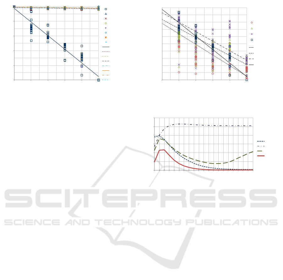
The results in Table 3 show that, in contrast to
what happens with the AoD ratio, the averages of
the levels of H2D, H3D, E2D, E3D, COS, VB-0 and
VB-1 are hardly affected by the variation of the per-
centage of opposites (see in Figure 4 the broad dif-
Choosing Suitable Similarity Measures to Compare Intuitionistic Fuzzy Sets that Represent Experience-Based Evaluation Sets
65

0
0.2
0.4
0.6
0.8
1
0 0.2 0.4 0.6 0.8 1
AoD
H2D
H3D
E2D
E3D
COS
VB-0
VB-1
LM(AoD)
LM(H3D)
LM(E2D)
LM(E3D)
LM(COS)
LM(H2D)
LM(VB-0)
LM(VB-1)
opposites (%)
similarity
Figure 4: Bivariate plots H2D-vs.-OP, H3D-vs.-OP, E2D-
vs.-OP, E3D-vs.-OP, COS-vs.-OP, vB-0-vs.-OP and VB-1-
vs.-OP in contrast to AoD-vs.-OP.
ference among the slopes of the linear models corre-
sponding to these similarity measures and the slope
of the linear model corresponding to the AoD ratio).
By way of illustration, if we use the resulting model
for COS (i.e., y = −0.0004x + 0.9831) to compute the
level to which the average of evaluations given under
the scenarios R0 and R100 are similar, we will ob-
tain y = 0.9827 as a result —since R100 contains the
100% of opposite training examples in relation to R0,
we fix x = 1 to make this computation. Notice that this
result, which is reflected by the lowest manifest index
(i.e., m = 0), differs markedly from the result obtained
for AoD (i.e., y = 0.0469). This means that, e.g., if
one of these (configurations of) similarity measures is
used in a clustering process to group evaluations given
by people with different knowledge (or understand-
ing) about a particular category, say E11, the evalua-
tions given by two persons having contradictory un-
derstandings of E11 will probably (and badly) be put
into the same group.
With respect to the averages of the levels of the
configurations related to (10), the results in Table 3
show that three of them, namely XVB-0-0.05, XVB-0-
0.1 and XVB-0.5-0.1, are fairly affected by the vari-
ation of the percentage of opposites (see Figure 5).
Notice that the correlations for XVB-0-0.05, XVB-0-
0.1 and XVB-0.5-0.1 (i.e., R = −0.8289, R = −0.8099
and R = −0.8294 respectively) denote fairly strong
negative relationships that are roughly comparable
with the strongly negative relationship (R = −0.9741)
in AoD-vs.-OP. To illustrate this, if the resulting
model for XVS-0-0.1 (i.e., y = −0.6587x + 0.6560) is
used in the above example (i.e., with x = 1), we will
obtain y = −0.0027 as a result, which is fairly close
to the result obtained for AoD (i.e., y = 0.0469).
Since (10) is based on the weight of a CDP and
the computation of this weight was based on the w-
parameter in our testing procedure (see Section 4.2.2),
0
0.2
0.4
0.6
0.8
1
0 0.2 0.4 0.6 0.8 1
opposites (%)
similarity
XVB-0-0.05
XVB-0.5-0.1
XVB-0-0.1
AoD
LM(XVB-0-0.05)
LM(XVB-0.5-0.1)
LM(XVB-0-0.1)
LM(AoD)
Figure 5: Bivariate plots XVB-0-0.05-vs.-OP, XVB-0-0.1-
vs.-OP and XVB-0.5-0.1-vs.-OP in contrast to AoD-vs.-OP.
0.0
0.2
0.4
0.6
0.8
1.0
1.2
0 0.1 0.2 0.3 0.4 0.5 0.6 0.7 0.8 0.9 1
w-parameter
m-index
a
SM
a
AoD
/
b
SM
b
AoD
/
R
SM
R
AoD
/
2
2
Figure 6: Influence of the w-parameter on the quality of the
m-index for XVB-0-w.
we performed additional tests to observe the influence
of this parameter on the quality of the results of this
similarity measure. In such additional tests, we con-
figured (10) with α = 0 and w = 0.05,0.1, 0.15,··· ,1
and used the same nomenclature (i.e., XVB-α-w) to
label each configuration. Figure 6 shows how the
m-index corresponding to the linear model for each
XVB-0-w-vs-OP relationship is affected by the w-
parameter. Notice that the peak m-index is reached
at w = 0.1 and is projected to decline after that point.
Recalling from Section 4.2.2, the w-parameter deter-
mines the wide of the average gap between the mem-
bership and non-membership values, which is then
used to build a CDP for the IFSs in the similarity
comparison as seen from the perspective of the per-
son who provides the referent IFS. This means that,
in this scenario, a spot difference with a magnitude
less than or equal to the 10% of the average gap be-
tween the membership and non-membership values
(see Sections 2.2.2 and 4.2.2) will roughly reflect a
similar understanding (or knowledge) of the evaluate
concept. This result seems to support the idea behind
a CDP, which suggests that “a difference in under-
standing of a concept could be marked by a difference
in one or more evaluations”(Loor and De Tr
´
e, 2014).
FCTA 2015 - 7th International Conference on Fuzzy Computation Theory and Applications
66

5.3 Discussion
The results suggest that only some of the configura-
tions of the similarity measure (10), namely XVB-0-
0.05, XVB-0-0.1 and XVB-0.5-0.1, reflect adequately
the perceived similarity between the simulated IFSs.
This means that, e.g., if you and a new coworker
have been individually asked to evaluate the level
to which several stories can be published in E11
and an experience-based clustering system has been
used with (10) to group similar evaluations, your
coworker’s evaluations and yours will be adequately
grouped. That is, if your coworker’s understand-
ing about E11 is very similar to your understanding,
the evaluations of you two will fairly put into the
same group; otherwise, they will be put into different
groups.
A possible explanation for those results might be
that, by means of the ∆
@A
, the similarity measure (10)
takes into account what is understood as a qualitative
difference between two IFS-elements from the per-
spective of the evaluator who provides the IFS A. This
situation is observable when the average gap between
the membership and non-membership components of
the IFS-elements in A is taken into account to com-
pute ∆
@A
= weightCDP(A,B, w) (see Equation (21)).
Since such an average gap could be very narrow in
the simulated IFSs (i.e., the average hesitation mar-
gin could be closer to the highest value), it might not
be taken into account by the other (configurations of)
similarity measures. In other words, the similarity
measure (10) seems to have the added advantage of
weighting a CDP between the IFSs involved in a sim-
ilarity comparison. If so, someone might ask: why not
using the weight of a CDP to extend the other simi-
larity measures and, thus, improve their results? An
answer might be: yes, it is an option but just keep in
mind that a CDP is directional, which contrasts with
the symmetric approach assumed in some similarity
measures (see Section 2.2).
Another possible explanation for the results might
be that a gap between the membership and non-
membership components is contextually related to the
categorization decision (see Sections 3.2.2 and 4.1),
which is deemed to be a point of reference for the per-
ceived similarity through the agreement on decision
ratio. Hence, a similarity measure such as (10) that
takes into account the aforesaid gap could reflect more
adequately the similarity perceived from the perspec-
tive of who makes the categorization decision.
Even though these results are based on simulated
IFSs that use a manually categorized newswire sto-
ries, they need to be interpreted with caution because
of the dependency of the IFSs with the learning algo-
rithm and the (text categorization) context that were
chosen for the simulations. Consequently, conducting
simulations with other learning algorithms and exper-
iments with real evaluators is recommended and sub-
ject to further study.
6 CONCLUSIONS
An experience-based evaluation is deemed to be a
judgment that depends on what each person has ex-
perienced or understood about a particular concept or
topic. Considering that such an evaluation could be
imprecise and marked by hesitation, in (Loor and De
Tr
´
e, 2014) the authors proposed modeling it as an el-
ement of an intuitionistic fuzzy set, or IFS for short
(Atanassov, 1986; Atanassov, 2012). This means that,
from a theoretical point of view, all the existing simi-
larity measures for IFSs could be used to compare two
experience-based evaluation sets.
To study empirically which similarity measures
for IFSs can actually be used to compare such IFSs,
in this paper we tested some of the existing similar-
ity measures in comparisons between pairs of IFSs
that result from simulations of experience-based eval-
uation processes. In such simulations we made use
of a learning algorithm that uses support vector ma-
chines (Vapnik, 1995; Vapnik and Vapnik, 1998) to
learn how a human editor categorizes newswire sto-
ries and, then, we made use of the resulting knowl-
edge to evaluate other stories.
The simulations were conducted under different
learning scenarios to observe how the chosen similar-
ity measures reflect the perceived similarity between
two IFSs that might be given by persons with differ-
ent background. A ratio that denotes how similar the
decisions are was deemed to be an indicator of the
perceived similarity.
The results suggest that the similarity measure
proposed in (Loor and De Tr
´
e, 2014), which takes into
account what is understood as a qualitative difference
between two IFS-elements by means of a connota-
tion differential print, could reflect more adequately
the perceived similarity. Consequently, this similarity
measure could potentially be used in a process such as
clustering or filtering of experience-based evaluations
given by people with different background, in which
a proper similarity comparison is needed —e.g., clus-
tering of evaluations given by residents about routes
in their city that are suitable for kids riding a bicycle.
However, the results need to be interpreted with
caution due to the dependency of the simulated IFSs
with the learning algorithm and the context that were
chosen for the simulations. Thus, conducting simula-
Choosing Suitable Similarity Measures to Compare Intuitionistic Fuzzy Sets that Represent Experience-Based Evaluation Sets
67

tions in other contexts with other learning algorithms
as well as conducting experiments with real evalua-
tors is recommended and subject to further study.
REFERENCES
Atanassov, K. T. (1986). Intuitionistic fuzzy sets. Fuzzy sets
and Systems, 20(1):87–96.
Atanassov, K. T. (2012). On Intuitionistic Fuzzy Sets The-
ory, volume 283 of Studies in Fuzziness and Soft Com-
puting. Springer Berlin Heidelberg, Berlin, Heidel-
berg.
Buckley, C., Salton, G., and Allan, J. (1994). The effect of
adding relevance information in a relevance feedback
environment. In Proceedings of the 17th Annual Inter-
national ACM SIGIR Conference on Research and De-
velopment in Information Retrieval, SIGIR ’94, pages
292–300, New York, NY, USA. Springer-Verlag New
York, Inc.
Burges, C. J. (1998). A tutorial on support vector machines
for pattern recognition. Data mining and knowledge
discovery, 2(2):121–167.
Joachims, T. (1998). Text categorization with support vec-
tor machines: Learning with many relevant features.
Springer.
Joachims, T. (1999). Making large-scale SVM learning
practical. In Sch
¨
olkopf, B., Burges, C., and Smola, A.,
editors, Advances in Kernel Methods - Support Vec-
tor Learning, chapter 11, pages 169–184. MIT Press,
Cambridge, MA.
Lewis, D. D., Yang, Y., Rose, T. G., and Li, F. (2004).
RCV1: A new benchmark collection for text catego-
rization research. The Journal of Machine Learning
Research, 5:361–397.
Loor, M. and De Tr
´
e, G. (2014). Connotation-differential
Prints - Comparing What Is Connoted Through
(Fuzzy) Evaluations. In Proceedings of the Interna-
tional Conference on Fuzzy Computation Theory and
Applications, pages 127–136.
Loor, M. and De Tr
´
e, G. (2014). Vector based similarity
measure for intuitionistic fuzzy sets. In Atanassov,
K. T., Baczy
´
nski, M., Drewniak, J., Kacprzyk,
J., Krawczak, M., Szmidt, E., Wygralak, M., and
Zadro
˙
zny, S., editors, Modern approaches in fuzzy
sets, intuitionistic fuzzy sets, generalized nets and re-
lated topics : volume I : foundations, pages 105–127.
SRI-PAS.
Rose, T., Stevenson, M., and Whitehead, M. (2002). The
reuters corpus volume 1-from yesterday’s news to to-
morrow’s language resources. In LREC, volume 2,
pages 827–832.
Szmidt, E. (2014). Similarity measures between intuition-
istic fuzzy sets. In Distances and Similarities in Intu-
itionistic Fuzzy Sets, volume 307 of Studies in Fuzzi-
ness and Soft Computing, pages 87–129. Springer In-
ternational Publishing.
Szmidt, E. and Kacprzyk, J. (2000). Distances between
intuitionistic fuzzy sets. Fuzzy Sets and Systems,
114(3):505–518.
Szmidt, E. and Kacprzyk, J. (2013). Geometric similarity
measures for the intuitionistic fuzzy sets. In 8th con-
ference of the European Society for Fuzzy Logic and
Technology (EUSFLAT-13), pages 840–847. Atlantis
Press.
Tversky, A. (1977). Features of similarity. Psychological
review, 84(4):327.
Vapnik, V. N. (1995). The nature of statistical learning the-
ory. Springer-Verlag New York, Inc.
Vapnik, V. N. and Vapnik, V. (1998). Statistical learning
theory, volume 1. Wiley New York.
Zadeh, L. (1965). Fuzzy sets. Information and control,
8(3):338–353.
FCTA 2015 - 7th International Conference on Fuzzy Computation Theory and Applications
68