Design of an Autonomous Intelligent Demand-Side Management System

by using Electric Vehicles as Mobile Energy Storage Units by Means of

Evolutionary Algorithms

Edgar Galv´an-L´opez

, Marc Schoenauer

and Constantinos Patsakis

School of Computer Science and Statistics, Trinity College Dublin, Dublin, Ireland

TAO Project, INRIA Saclay & LRI - Univ. Paris-Sud and CNRS, Orsay, France

Department of Informatics, University of Piraeus, Piraeus, Greece

Keywords:

Demand-Side Management, Electric Vehicles, Evolutionary Algorithms, Differential Evolution.

Abstract:

Evolutionary Algorithms (EAs), or Evolutionary Computation, are powerful algorithms that have been used in

a range of challenging real-world problems. In this paper, we are interested in their applicability on a dynamic

and complex problem borrowed from Demand-Side Management (DSM) systems, which is a highly popular

research area within smart grids. DSM systems aim to help both end-use consumer and utility companies

to reduce, for instance, peak loads by means of programs normally implemented by utility companies. In

this work, we propose a novel mechanism to design an autonomous intelligent DSM by using (EV) electric

vehicles’ batteries as mobile energy storage units to partially fulﬁll the energy demand of dozens of household

units. This mechanism uses EAs to automatically search for optimal plans, representing the energy drawn from

the EVs’ batteries. To test our approach, we used a dynamic scenario where we simulated the consumption of

40 and 80 household units over a period of 30 working days. The results obtained by our proposed approach

are highly encouraging: it is able to use the maximum allowed energy that can be taken from each EV for each

of the simulated days. Additionally, it uses the most amount of energy whenever it is needed the most (i.e.,

high-peak periods) resulting into reduction of peak loads.

1 INTRODUCTION

Evolutionary Algorithms (EAs) (B¨ack et al., 1999;

Eiben and Smith, 2003), also known as Evolution-

ary Computation systems, are inﬂuenced by the the-

ory of evolution by natural selection. These algo-

rithms have been with us for some decades and are

very popular due to robust theoretical work developed

around them that have helped us to understand why

they work (e.g, representations’ properties (Galv´an-

L´opez et al., 2010a; Fagan et al., 2010; Galv´an-L´opez

et al., 2008; McDermott et al., 2010)) and to due to

their successful application in a variety of different

problems, ranging from the automated design of an

antenna carried out by NASA (Lohn et al., 2005), the

automated optimisation of game controllers (Galv´an-

L´opez et al., 2010b), the automated evolution of Java

code (Cody-Kenny et al., 2015), to automated design

of combinational logic circuits (Galv´an-L´opez et al.,

2004; Galv´an-L´opez, 2008). EAs can be considered

a “black-box”, as they do not require any speciﬁc

knowledge of the ﬁtness function. They work even

when, for example, it is not possible to deﬁne a gradi-

ent on the ﬁtness function or to decompose the ﬁtness

function into a sum of per-variable objective func-

tions.

In this work, we are interested in investigating the

applicability of EAs in a dynamic and challenging

problem in Demand-Side Management (DSM) Sys-

tems taken from Smart Grids where, in summary, the

goal is to automatically create ﬁne-grained solutions

that indicate the amount of energy that can be taken

from electric vehicles’ (EVs) batteries to partially sat-

isfy energy demand in residential areas and reducing

electricity peaks, whenever possible. The proposed

approach and ﬁtness functions used in our work (de-

scribed in Section 2) is not amenable to analytic so-

lution or simple gradient-based optimisation, hence

search algorithms such as EAs are required.

DSM is normally considered as a mechanism

or program, implemented by utility companies, to

control the energy consumption at the customer

side (Masters, 2004). DSM is an important research

106

Galván-Lopez, E., Schoenauer, M. and Patsakis, C..

Design of an Autonomous Intelligent Demand-Side Management System by using Electric Vehicles as Mobile Energy Storage Units by Means of Evolutionary Algorithms.

In Proceedings of the 7th International Joint Conference on Computational Intelligence (IJCCI 2015) - Volume 1: ECTA, pages 106-115

ISBN: 978-989-758-157-1

area in the Smart Grid (SG) community as shown by

the increasing number of publications over the years

(e.g., more than 2,000 papers have been published in

this area where more than two thirds have been pub-

lished since 2010 (Galv´an-L´opez et al., 2014)). A vi-

sual representation of the research conducted in DSM

over the last years can be found in (Galv´an-L´opez

et al., 2015).

DSM programs include different approaches (e.g.,

manual conservation and energy efﬁciency pro-

grams (pen, 2007), Residential Load Management

(RLM) (Galvan et al., 2012; Mohsenian-Rad et al.,

2010)), where RLM programs based on smart pric-

ing are amongst the most popular methods. The idea

behind smart pricing is to encourage users to manage

their loads, so that they can reduce electricity prices

while, at the same time, the utility companies achieve

a reduction in the peak-to-average ratio (PAR)

load demand by shifting consumption whenever pos-

sible (Galvan et al., 2012; Galv´an-L´opez et al., 2014).

One of the major limitations of smart pricing is

the fact that the electricity price is proportional to

the electricity demand (i.e., a high number of appli-

ances/devices connected to the grid results in hav-

ing high electricity costs). To alleviate this problem,

we propose the development of a demand-side au-

tonomous intelligent management system that exploit

electric vehicles’ (EV) batteries. More precisely, our

system uses the EV’s batteries to partially and tem-

porarily fulﬁll the demand of end-use consumers in-

stead of using only the electricity available from a

substation transformer. This is possible thanks to the

vehicle to grid (V2G) technology, which is described

as a system in which electric-drive vehicles can feed

power to the grid with the appropriate communica-

tion/connection technologies acting as mobile gener-

ators of limited output (Kempton and Letendre, 1997;

Kempton and Tomic, 2005).

The deployment of such a system implies several

signiﬁcant challenges, e.g. different driving patterns

resulting in the amount of energy needed at the time

of departure, amount of energy taken from the EVs’

batteries. To tackle this problem, we use an optimisa-

tion EA.

Thus, the main contribution of this research is

a novel approach to balance the load demand from

dozens of household units using both a substation

transformer and EVs’ batteries as mobile energy stor-

age units

by considering the automatic generation of

Peak-to-average ratio is calculated by the maximum

load demand for a period of time over the average load

demand, so a lower PAR is normally preferred due to e.g.

maintenance costs (Mohsenian-Rad et al., 2010).

In this work, we use the terms “substation trans-

solutions via the use of EAs. To this end, we are in-

terested in maximising, in general, the use of avail-

able energy from the EVs’ batteries while ensuring

that each of the EVs can complete a journey to work,

where the EVs can be charged, and in particular, help-

ing in the reduction of peak loads at the transformer

level by using the most quantity of energy from the

EVs’ batteries. This problem would be simple enough

if it was not for the dynamicity associated to the prob-

lem and if we would not care about keeping the PAR

relatively low.

To achieve this, we allow the DSM system to

make ﬁne-grained decisions (i.e., variable amount of

energy requested) by using a continuous representa-

tion instead of using a discrete representation (i.e.,

turning a device/appliance on or off resulting in feed-

ing/getting a constant amount of energy) as normally

adopted in DSM (Brooks et al., 2010).

To this end, we use a form of EAs, called Dif-

ferential Evolution (DE) (Storn and Price, 1997), that

allows us to achieve this. More speciﬁcally, DE uses

a vector of real-valued functions and we use them to

represent an individual (potential solution) that speci-

ﬁes an energy consumption scheduling vector, which

in turn indicates the amount of energy that should be

taken from the EVs’ batteries aiming at fulﬁlling the

goals previously described (e.g., maximising the en-

ergy consumption availablefrom the batteries while at

the same time reducing peak loads at the transformer

level with associated constraints such as guaranteeing

that each EV would complete a journey to work). De-

tails on how this algorithm works and its adoption in

this research are described in Section 2.

The rest of this paper is organised as follows. In

the following section we introduce DE and present

our proposed approach. In Section 3, we present the

experimental setup used in this work and Section 4

discusses the ﬁndings of our approach. Finally, in

Section 5 we draw some conclusions.

2 PROPOSED APPROACH

2.1 Background

There are multiple EAs methods, such as Genetic

Algorithms (GAs) (Goldberg, 1989), Genetic Pro-

gramming (GP) (Koza, 1992), Differential Evolution

(DE) (Storn and Price, 1997). All these methods use

evolution as an inspiration to automatically generate

potential solutions for a given problem. They differ,

former” and “EV’s batteries” to differentiate between the

two sources of energy.

Design of an Autonomous Intelligent Demand-Side Management System by using Electric Vehicles as Mobile Energy Storage Units by

Means of Evolutionary Algorithms

107

mainly, in the representation used (i.e., encoding of

a solution). For example, the typical representation

used in GAs is ﬁxed bitstrings, GP’s typical repre-

sentation is tree-like structures, DE uses a vector of

real-valued functions.

In this work, we use a DE algorithm given its nat-

ural representation (i.e., real-valued functions). Other

bio-inspired algorithms can also use this type of rep-

resentation, however, in this work we decided to use a

DE given its efﬁciency for global optimisation over

continuous search spaces (Storn and Price, 1997).

By using this type of representation, we can have

a more ﬁne-grained action granularity (e.g., in this

work, each element in the vector represents how much

energy will be taken from the EVs’ batteries to feed

household units), instead of using a more limited

representation such as a bitstring representation that

could indicate to take a pre-deﬁned amount of energy

(i.e., on or off) from EVs’ batteries to partially fulﬁll

energy consumption from household units. We fur-

ther discuss this later in this section.

The goal of DE is to evolve NP D-dimensional

parameter vectors x

i,G

= 1, 2, ··· , NP, so-called pop-

ulation, which encode the potential solutions (indi-

viduals), i.e., x

i,G

= {x

i,G

··· , x

i,G

}, i = 1, · ·· , NP to-

wards the global optimum solution (e.g., highest val-

ues when maximising a cost function). The initial

population is randomly generated and this should be

done by spreading the points across the entire search

space (e.g., this could be achievedby distributingeach

parameter on an individual vector with uniform dis-

tribution between lower and upper bounds x

and x

To automatically evolve these potential solutions over

generations via the deﬁnition of a ﬁtness function, DE

uses the most common bio-inspired operators as com-

monly carried out in EAs: mutation and crossover to

ﬁnd the global optimum solution. Each of these oper-

ators is brieﬂy explained in the following lines (refer

to (Qin et al., 2009; Storn and Price, 1997) for a de-

tailed description on how they work).

The mutation operator generates a mutant vector

following one of the following strategies:

DE/rand/1

i,G

= x

+ F ·(x

− x

)

DE/best/1

i,G

= x

best,G

+ F ·(x

− x

)

DE/rand-to-best/1

i,G

= x

i,G

+ F ·(x

best,G

− x

i,G

) + F · (x

− x

)

DE/best/2

i,G

= x

best,G

+ F ·(x

− x

) + F · (x

− x

)

DE/rand/2

i,G

= x

+ F ·(x

− x

) + F · (x

− x

)

where indexes r

, r

∈ {1, 2, ··· , NP} are ran-

dom and mutually different. F is a real and con-

stant factor ∈ [0, 2] for scaling differential vectors and

best,G

is the individual with best ﬁtness value (e.g.,

highest value for a maximisation function) in the pop-

ulation at generation G.

The crossover operator increases the diversity of

the mutated parameter vectors and is deﬁned by:

i,G+1

= (v

1i,G+1

, v

2i,G+1

, ··· , v

Di,G+1

)

where:

ji,G+1



ji,G+1

if randb( j) ≤ CR or j = rnbr(i),

ji,G

otherwise

where j = 1, ·· · , D, randb( j) is the j

evaluation of

a uniform random number generator with outcome

∈ [0, 1]. CR is the constant crossover rate ∈ [0, 1].

rnbr(i) is a randomly chosen index ∈ 1, 2, · ·· , D

which ensures that u

i,G+1

receives at least one param-

eter value from u

i,G+1

The performance of the DE algorithm depends on

different factors, such as the values associated to the

parameters (e.g., population size) as well as the vari-

ant of the operator used (e.g., variant of the muta-

tion operator). This, intuitively means, that some pre-

liminary runs would be normally required to deter-

mine which variant of an operator performs better on

a given problem. We further discuss this in the fol-

lowing section.

2.2 Proposed Representation and

Fitness Function

We nowextend the natural DE representationto tackle

the problem described throughout the paper and pro-

ceed to deﬁne the ﬁtness function (cost function) that

allows the algorithm to automatically guide the evo-

lutionary search.

Let N denote the number of household units

(users), where the number of household units is N ,|

N |. For each household n ∈ N, let l

denote the total

load at time t ∈ T , {t

, ··· , t

}. Without loss of gen-

erality, we assume that time granularity is 15 minutes.

The load for household n, from t

to t

, is denoted by:

, [l

, ··· , l

] (1)

From this, we can calculate the load across all

household units N at each time t ∈ [t

] as follows:

∑

n∈N

(2)

ECTA 2015 - 7th International Conference on Evolutionary Computation Theory and Applications

108

Similarly, let M denote the number of electric ve-

hicles available in N. For each electric vehicle m ∈ M,

let E

denote the energy that can be taken from the

EV at time t ∈ T , {t

, ··· , t

}. Without loss of gen-

erality, we assume that time granularity is again 15

minutes. The total energy taken from an EV from t

until t

is denoted by:

, [E

, ··· , E

] (3)

We use this as a foundation to represent an indi-

vidual that speciﬁes an energy consumption schedul-

ing vector. More speciﬁcally, an individual is repre-

sented by:







, ··· , E







(4)

where each E

is a real value representing the amount

of energy taken from an EV’s battery. Each row rep-

resents the behaviour of a single EV over the full pe-

riod; each column represents the behaviour of all EVs

at a single time-slot. An individual in the EA is just

a matrix E

, unrolled to give a vector of real-valued

functions, that is:

, ··· , E

, E

, ··· , E

(5)

Based on these deﬁnitions, the total energy taken

across all M EVs at each t ∈ [t

] can be calculated

as:

∑

m∈M

(6)

To automatically ﬁnd good energy consumption

scheduling solutions, deﬁned in Equation 4, we need

to deﬁne a ﬁtness function (cost function) that indi-

cates the quality of our evolved solution. First, we

focus our attention in designing a cost function that

tries to create valid solutions in terms of using the

maximum allowed energy from each EV (i.e., guar-

anteeing that a minimum state of charge (SoC) is left

at the time of departure t

From Equation 3, we know the amount of energy

available from m ∈ M at any given period of time t

denoted by E

. Because each EV can be charged at

work and the distance from home to work remains

constant, it is fair to assume the knowledge of a

minimum SoC expressed in kW, denoted as m

SoC

, at

the time of departure t

for each m ∈ M, so that it can

reach work and be recharged at a lower rate. From

this, we let the DE to assess a potential solution,

denoted in Equation 4, measuring the amount of

energy taken from the EVs.

This is deﬁned as:

) , maximise

#{m ∈ M}

∑

m∈M

+ (E

+ 1)(m

SoC

− E

)

SoC



− m

SoC



(7)

Equation 7 guides evolutionary search towards a

local optimum solution since it only encourages the

ﬁnding of solutions that maximise the use of allow-

able energy taken from EVs’ batteries. Thus, there is

a necessity to further enrich this equation, so that a

higher quantity of energy is taken from the EVs’ bat-

teries whenever deemed necessary (e.g., higher con-

sumption during high peak periods). We achieve this

by using Equations 2 and 6 that indicate the load

across all household units L

at time t and the total

energy taken across all EVs E

at time t, respectively;

and we deﬁne a degree of importance for each time

slot as t

. Putting everything together we have:

) , f

) + maximise

#{m ∈ M}

∑

t=t

∀t

< T

−

#{m ∈ M}

∑

t=t

∀r ≥ T

(8)

where T

is a threshold that denotes the number of

time slots that are considered critical (i.e., high peak

period). In this work, as deﬁned in this section and

we discuss further afterwards, a number of time slots

is deﬁned by t

and t

, where a third is considered

critical (T

= 20).

3 EXPERIMENTAL SETUP

3.1 Household Units

To test the scalability of our proposed approach, we

simulated the consumption of 40 and 80 household

units, where each of them uses between 10 and 20

appliances. As indicated throughout the paper, the

goal is to use EVs’ batteries in an intelligent way to

partially satisfy energy demand from the end-use con-

sumers (recall that we work under the assumption that

the EVs can be charged at work).

To this end, we simulated that around 20% of

household units account for an EV. To makethis prob-

lem dynamic, we allowed the patterns of arrival (t

departure (t

) and initial State of Charge (SoC) for

each of the EVs to vary for each of the 30 simulated

working days. More speciﬁcally, the arrival and de-

parture time for each of the EVs have a 90-minute

Design of an Autonomous Intelligent Demand-Side Management System by using Electric Vehicles as Mobile Energy Storage Units by

Means of Evolutionary Algorithms

109

time frame starting at t

=17:00 and t

=6:30, respec-

tively (i.e., arrival time could be between 17:00 and

18:30, whereas departure time could be between 6:30

and 8:00). The initial SoC

for each of the EVs for

each of the simulated days is set between 48% and

60% and the ﬁnal SoC

is set between 30% and 35%

to allow each EV to reach work. Table 1 summarises

the parameters used to simulate our scenario. We ran

our simulations for a period of 30 days of simulated

time.

3.2 Scenarios

As indicated in Section 2, we deﬁned a bottom-up

approach, where we deﬁned, ﬁrst, a ﬁtness function

that tries to maximise the energy that can be taken

from the EVs’ batteries while ensuring that each of

them reaches work, described in Equation 7, and then

we enriched the ﬁtness function by trying to also re-

duce the highest load demands at the substation trans-

former, described in Equation 8 (i.e., use the most

amount of energy from the batteries at high-peak time

while at the same time ensuring the PAR remains

low). We tested both ﬁtness functions for 40 and 80

household units, resulting in four different scenarios.

3.3 Differential Evolution

As mentioned in Section 2, differential evolution’s

performance, as any other evolution-based algorithm,

depends, among other things, on the values associ-

ated to the parameters that need to be speciﬁed for

the algorithm (e.g., population size, number of gener-

ations), in general, and in the type of operator used, in

particular.

No a priori knowledge is available to presume

which mutation operator will perform better in the

previously deﬁned problem. To this end, we exe-

cuted 30 independent runs of our proposed approach

for each of the mutation variants, e.g., DE/rand/1,

DE/best/1, (150

independentruns in total to ﬁnd only

the best mutation strategy) using the ﬁrst proposed ﬁt-

ness function (Equation 7) which maximises the en-

ergy taken from 11 EVs’ batteries to complement the

energy consumption of 40 household units averaged

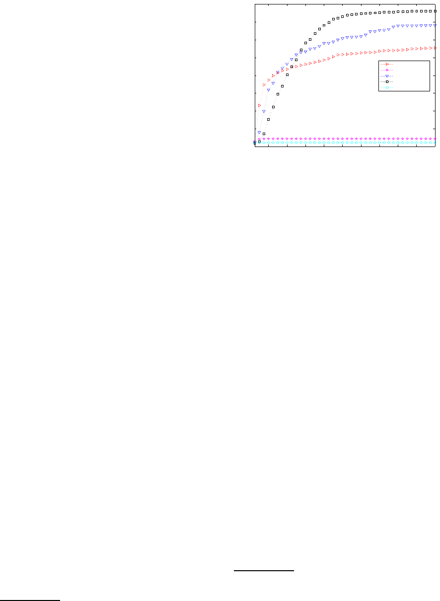
over 30 days. Figure 1 shows the performance by

measuring the average of best ﬁtness per generation

for each of the ﬁve mutation variants, using a popula-

tion size of 500 individuals and 200 generations.

Clearly, the mutation strategy DE/rand/2 achieved

the best performance and we used it to run our exper-

iments to automatically ﬁnd a (nearly) optimal solu-

30 independent runs * 5 variants of the mutation oper-

ator.

20 40 60 80 100 120 140 160 180 200

0.2

0.3

0.4

0.5

0.6

0.7

0.8

0.9

Number of generations

Average of best fitness

DE/best/1

DE/best/2

DE/rand/1

DE/rand/2

DE/rand−to−best/1

Figure 1: Average of best ﬁtness values of 30 independent

runs for each of the ﬁve types of mutation operators tested

in this work, using 500 individuals and 200 generations, to

maximise energy consumption from electric vehicles’ bat-

teries (Equation 7). Higher values are preferred.

tion. To obtain meaningful results, we performed 30

independent runs for each of the scenarios explained

in the previous paragraphs (we executed 30 * 4 runs in

total

). Runs were stopped when the maximum num-

ber of generations was reached.

As mentioned in Section 2, every element of the

DE vector represents how much energy can be taken

from the batteries of the EVs. We make a decision ev-

ery 15 minutes. Thus, the length of the individual that

represent the solution is the number of time slots de-

ﬁned between 17:00 and 8:00am, whereas the height

is deﬁned by the number of electric vehicles used, as

deﬁned in Equation 4. The parameters used in our

experiments are summarised in Table 2.

4 RESULTS

In the following paragraphs, we will analyse: (a) how

the EVs’ batteries were used to partially satisfy the

demand of a set of household units, (b) when the high-

est consumption from EVs’ batteries occurred, and

ﬁnally, (c) the implications of the new consumption

model via the analysis of the peak-to-average-ratio.

4.1 Maximising Energy Consumption

from EVs’ batteries

Let us start analysing our approach on how the

30 independent runs, 4 different scenarios (i.e., 40 and

80 household units, trying to maximise: (a) energy con-

sumption from EVs, and (b) energy consumption from EVs

considering reducing highest load peaks; for each of the set

of household units used in this work).

ECTA 2015 - 7th International Conference on Evolutionary Computation Theory and Applications

110

Table 1: Summary of parameters used for our smart grid

system.

Parameter Value

Number of household units 40, 80

Number of appliances Uniform in [10,20]

Number of EVs ≈ 20% of houses

have one EV

Arrival and departure time t

=[17:00,18:30]

=[6:30,8:00]

Frequency of making a decision 15 minutes

Number of times slots T 60

State of Charge at t

Uniform in [48, 60]

State of Charge at t

Uniform in [30, 35]

Table 2: Summary of parameters used for our evolution-

ary algorithm.

Parameter Value/Comment

Population size 500

Length of the chromosome T (see Table 1)

Height of the chromosome Number of EVs

(see Table 1)

Generations 200

Crossover rate 0.5

Mutation strategy DE/rand/2

Termination criterion Maximum number

of generations

Independent runs 30

batteries of the EVs helped to partially satisfy the con-

sumption demand from a set of household units. The

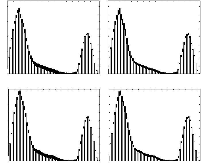
averaged consumption over a period of 30 days of

these household can be seen in Figure 2 (a, b) and

(c, d) for 40 and 80 houses, respectively.

In the left-hand side of this ﬁgure, we show the

distribution of consumption of both transformer and

EVs’ batteries proposed by the differential evolution

algorithm, when trying to maximise the consumption

of energy from the EVs’ batteries via Equation 7.

More speciﬁcally, it aims at using all the possible en-

ergy available from the batteries while guaranteeing

that each EV has a minimal SoC at the time of depar-

ture (see Table 1) that guarantees that each EV will

reach work. The white-ﬁlled bars represent the en-

ergy taken from the substation transformer whereas

the remaining energy consumption to fulﬁll the en-

ergy demand is taken from the EVs’ batteries. The

latter is shown by the black-ﬁlled bars.

Because we are interested in using the EVs’ bat-

teries as mobile energy storage units, we are partic-

ularly interested in seeing how the energy consump-

tion from these is managed by the differential evo-

lution algorithm. In the ﬁrst instance of our algo-

rithm (i.e., maximising the energy consumption from

the batteries of EVs with associated constraints, as

mentioned previously), it is expected that the energy

taken from the batteries would not follow a particu-

lar pattern (e.g., there is no correlation between the

amount of energy consumption from EVs and the en-

ergy needed by a number of household units). Indeed,

this is the case as seen in the left-hand side of Fig-

ure 2. For example, notice how the consumption from

EVs’ is proportionally similar during both high-peak

(e.g., 18:30 - 19:30) and low-peak periods (e.g., 22:00

- 23:00).

The situation is more encouraging when we con-

sider the second instance of our algorithm (i.e.,

maximising energy consumption from EVs’ batteries

while considering high-peak periods), shown in the

right-hand side of Figure 2. As it can be observed, the

proposed enriched ﬁtness function, shown in Equa-

tion 8, is able to automatically produce results that

can reduce the load peaks from the substation trans-

former by using more electricity from the EVs’ bat-

teries. For example, notice how the consumption of

energy from batteries is higher during high-peak pe-

riods (e.g., 18:30 - 19:30) and lower during low-peak

periods (e.g., 22:00 - 23:00).

4.2 Consumption from EV’s batteries

In the previous paragraphs, we discussed and showed

the results obtained by our approach using two cost

functions, formally described in Equations 7 and 8.

It is clear that the latter function is able to use a

higher quantity of energy from the EVs’ batteries dur-

ing high-peak periods compared to the effects when

using the former function, as shown in the right-hand

and left-hand side of Figure 2, respectively, using 40

and 80 household units. This averaged result over a

period of 30 simulated working days, however, does

not inform us in detail when the highest consumption

from batteries occurred (e.g., when and how much

consumption from the batteries for every of the simu-

lated days occurred).

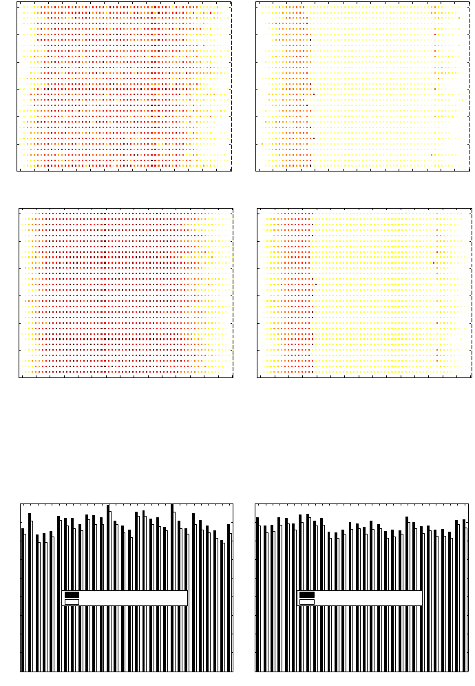
To this end, we kept track of the consumption

from the EVs’ batteries during the simulated period of

time (i.e., 17:00 - 8:00) for every day of the simulated

days. The patterns of such consumption are shown

in Figure 3 (a, b) and (c, d) for 40 and 80 household

units, respectively.

Let us start our analysis when maximising the en-

ergy that can be taken from the batteries while ensur-

ing that each EV has the minimum SoC at the time

of departure, deﬁned in Equation 7. The consump-

tion pattern of this is shown in Figure 3 (a) and (c) for

40 and 80 household units, respectively. It should be

noted that the higher the consumption from batteries

is, the darker the dot. We can see that a random pat-

tern is achieved by the cost function shown in Equa-

tion 7. That is, for every recorded day, shown in the y-

Design of an Autonomous Intelligent Demand-Side Management System by using Electric Vehicles as Mobile Energy Storage Units by

Means of Evolutionary Algorithms

111

17 18 19 20 21 22 23 0 1 2 3 4 5 6 7 8

Time of day (15 mins. granularity)

Consumption (kWh)

17 18 19 20 21 22 23 0 1 2 3 4 5 6 7 8

Time of day (15 mins. granularity)

Consumption (kWh)

(a) (b)

17 18 19 20 21 22 23 0 1 2 3 4 5 6 7 8

100

120

140

160

Time of day (15 mins. granularity)

Consumption (kWh)

17 18 19 20 21 22 23 0 1 2 3 4 5 6 7 8

100

120

140

160

Time of day (15 mins. granularity)

Consumption (kWh)

Figure 2: Average of 30-day energy consumption for 40 (top) and 80 (bottom) household units, each using between 10-20

appliances. The consumption of energy from the transformer alone is shown by the white-ﬁlled bars whereas the black-ﬁlled

bars represent the consumption taken from electric vehicles’ batteries. Maximising energy consumption from electric vehicles

only and maximising energy consumption from electric vehicles considering reducing highest load peaks are shown in the

left-hand side and right-hand side of the ﬁgure, respectively.

axis, the amount of energy taken from the batteries is

rather random regardless of the period time, shown in

the x-axis, except from 17:00-18:30 and 6:30 – 8:00,

where the consumption from batteries is low. This

can be explained due to the availability of EVs during

these periods. That is, as indicated in Section 3, each

EV has its own time of arrival and departure which

varies during these periods of time.

We continue our analysis on the proposed en-

riched maximisation cost function, see Equation 8,

that aims at using the most amount of energy from

the batteries of the EVs while ensuring that each has a

minimum SoC at the time of departure, and that tries

to reduce the highest peak loads. The consumption

pattern from the batteries is shown in Figure 3 (b) and

(d) for 40 and 80 household units, respectively. This

is a mirror image of what we discussed in the previ-

ous paragraph. That is, there is a well-deﬁned pattern

for each of the simulated days, shown in the y-axis,

during the period of study, shown in the x-axis of the

ﬁgure. We can observe that this cost function indeed

achievesat using the most amount of energy when it is

needed the most (high-peaks) as shown by the darker-

ﬁlled squares while ensuring that the constraints are

not violated (e.g., minimum SoC at the time of depar-

ture).

4.3 Peak-To-Average Ratio

As indicated previously, the peak-to-average ratio

(PAR) is calculated by the maximum load demand for

a period of time over the average load demand for the

same period. It has been shown that a lower PAR is

preferred (Mohsenian-Rad et al., 2010).

We calculated the PAR considering the consump-

tion from the substation transformer. Figure 4 shows

the PAR for 40 (left-hand side) and 80 (right-hand

side) household units for each of the 30 working sim-

ulated days using our proposed approach. It is easy to

observe that a higher PAR is achieved by the ﬁtness

(cost) function formally deﬁned in Equation 7, which

goal is to use the most amount of energy from EVs’

batteries while at the same time aims at guaranteeing

that each EV has a minimum SoC at the time of depar-

ECTA 2015 - 7th International Conference on Evolutionary Computation Theory and Applications

112

17 18 19 20 21 22 23 0 1 2 3 4 5 6 7 8

Time of day (15 mins. granularity)

Days

17 18 19 20 21 22 23 0 1 2 3 4 5 6 7 8

Time of day (15 mins. granularity)

Days

(a) (b)

17 18 19 20 21 22 23 0 1 2 3 4 5 6 7 8

Time of day (15 mins. granularity)

Days

17 18 19 20 21 22 23 0 1 2 3 4 5 6 7 8

Time of day (15 mins. granularity)

Days

Figure 3: Energy quantity taken from 11 (a, b) and 21 (c, d) electric vehicles over the range of time period studied in this

work, from 17:00 until 8:00 (shown in the x-axis), for 30 days (shown in the y-axis) to help with the energy consumption of

40 (a, b) and 80 (c, d) household units. Darker-ﬁlled circles represent higher energy quantity taken from the EVs’ batteries.

The enriched cost function, described in Equation 8, follows a well-deﬁned desired pattern (b, d), whereas the cost function

that tends to ﬁnd local optimum solutions, described in Equation 7, tends to have a rather undesirable random pattern (a, c).

1 2 3 4 5 6 7 8 9 10 11 12 13 14 15 16 17 18 19 20 21 22 23 24 25 26 27 28 29 30

0.5

1.5

2.5

3.5

4.5

Day

Peak−to−average ratio

Optimising consumption of energy battery

Optimising reduction of highest electricity peaks

1 2 3 4 5 6 7 8 9 10 11 12 13 14 15 16 17 18 19 20 21 22 23 24 25 26 27 28 29 30

0.5

1.5

2.5

3.5

4.5

Day

Peak−to−average ratio

Optimising consumption of energy battery

Optimising reduction of highest electricity peaks

Figure 4: Peak-to-average ratio (PAR) load demand achieved by our proposed approach when trying to maximise energy

consumption from EVs’ batteries (black-ﬁlled bars) vs. when trying to maximise energy consumption from EVs’ batteries

while aiming at reducing highest load peaks (white-ﬁlled bars), for 40 and 80 household units shown at the left-hand side and

right-hand side of the ﬁgure, respectively. A lower PAR is preferred.

ture compared to that PAR achieved by the enriched

ﬁtness function formally described in Equation 8 that

is built on the top of Equation 7, which also tries to

reduce the highest peak loads.

This, in fact, is to be expected given that the ﬁtness

function described in Equation 8 does consider an as-

sociated ranking system (recall that a third of time

slots are considered critical, i.e., high peak period)

that is able to reﬂect smoothly the consumption from

the substation transformer as shown by the low PAR

achievedby this enriched ﬁtness function for each day

of the 30 simulated days, denoted by the white-ﬁlled

Design of an Autonomous Intelligent Demand-Side Management System by using Electric Vehicles as Mobile Energy Storage Units by

Means of Evolutionary Algorithms

113

bars in Figure 4.

5 CONCLUSIONS

Evolutionary Algorithms are very popular given its

applicability in a range of static problems. In this

work, we focus our attention on using a differen-

tial evolution (DE) algorithm in a fairly complex and

dynamic problem taken from Demand-Side Manage-

ment (DSM) systems. DSM systems play an impor-

tant role in the SG. Their importance can be under-

stood by considering the new challenges that are con-

tinuously introduced to the grid, for example, electric

appliances that could double the average household

(e.g., electric vehicles). The correct design of a DSM

manages to use the available energy efﬁciently, with-

out the necessity of installing new electricity infras-

tructure.

In the specialised literature, there are several tech-

niques adopted by DSM programs. Perhaps, the most

popular techniques are those inspired on smart pric-

ing. Brieﬂy, the idea is to incentivise end-consumers

to shift energy consumption to hours when the elec-

tricity price is low, reducing both electricity costs and

energy-load consumption.

We believe that another important research area

worth exploring in DSM is to exploit “new” avail-

able technologies. In particular, we regard that there

is a lot of potential in utilising EVs’ batteries as mo-

bile energy storage units. To this end, we propose

a demand-side autonomous intelligent management

system that uses them to partially fulﬁll the demand of

end-use consumers instead of using only the electric-

ity available from a substation transformer, whenever

possible. To this end, we use a DE algorithm, that

is able to automatically create ﬁne-grained solutions

that indicate the amount of energy that can be taken

from the EVs, rather than adopting a more constraint

representation (e.g., on/off of EVs).

The results achieved by our proposed approach

are highly encouraging. That is, we showed how DE

is able to correctly use the maximum amount of en-

ergy while ensuring a minimum SoC for each EV for

each day of the 30 simulated working days. We built

upon this to automatically ﬁnd the best possible con-

ﬁguration of values (i.e., consumption from batteries)

whenever it was needed the most (i.e., high-peaks),

while simultaneously, demonstrating that it was pos-

sible to do so by keeping the PAR low.

ACKNOWLEDGEMENTS

Edgar Galv´an L´opez’s research is funded by an ELE-

VATE Fellowship, the Irish Research Council’s Ca-

reer Development Fellowship co-funded by Marie

Curie Actions. The ﬁrst author would also like to

thank the TAO group at INRIA Saclay & LRI - Univ.

Paris-Sud and CNRS, Orsay, France for hosting him

during the outgoing phase of the ELEVATE Fellow-

ship. The authors would like to thank all the review-

ers for their useful comments that helped us to signif-

icantly improve our work.

REFERENCES

(2007). Paciﬁc Northwest GridWise Testbed Demonstration

Projects, Part I. Olympic Peninsula Project.

B¨ack, T., Fogel, D. B., and Michalewicz, Z., editors (1999).

Evolutionary Computation 1: Basic Algorithms and

Operators. IOP Publishing Ltd., Bristol, UK.

Brooks, A., Lu, E., Reicher, D., Spirakis, C., and Weihl, B.

(2010). Demand dispatch: Using real-time control of

demand to help balance generation and load. IEEE

Power & Energy Magazine,, 8:20 – 29.

Cody-Kenny, B., Galv´an-L´opez, E., and Barrett, S. (2015).

locogp: Improving performance by genetic program-

ming java source code. In Proceedings of the Com-

panion Publication of the 2015 on Genetic and Evolu-

tionary Computation Conference, GECCO Compan-

ion ’15, pages 811–818, New York, NY, USA. ACM.

Eiben, A. E. and Smith, J. E. (2003). Introduction to Evolu-

tionary Computing. Springer Verlag.

Fagan, D., ONeill, M., Galv´an-L´opez, E., Brabazon,

A., and McGarraghy, S. (2010). An analysis of

genotype-phenotype maps in grammatical evolution.

In Esparcia-Alczar, A., Ekrt, A., Silva, S., Dignum, S.,

and Uyar, A., editors, Genetic Programming, volume

6021 of Lecture Notes in Computer Science, pages

62–73. Springer Berlin Heidelberg.

Galvan, E., Harris, C., Dusparic, I., Clarke, S., and Cahill,

V. (2012). Reducing electricity costs in a dynamic

pricing environment. In Proc. Third IEEE Interna-

tional Conference on Smart Grid Communications

(SmartGridComm), pages 169 – 174, Tainan, Taiwan.

IEEE Press.

Galv´an-L´opez, E. (2008). Efﬁcient graph-based genetic

programming representation with multiple outputs.

International Journal of Automation and Computing,

5(1):81–89.

Galv´an-L´opez, E., Curran, T., McDermott, J., and Car-

roll, P. (2015). Design of an autonomous intelligent

demand-side management system using stochastic op-

timisation evolutionary algorithms. Neurocomputing,

170:270–285.

Galv´an-L´opez, E., Dignum, S., and Poli, R. (2008).

The effects of constant neutrality on performance

and problem hardness in gp. In Proceedings of

ECTA 2015 - 7th International Conference on Evolutionary Computation Theory and Applications

114

the 11th European conference on Genetic program-

ming, EuroGP’08, pages 312–324, Berlin, Heidel-

berg. Springer-Verlag.

Galv´an-L´opez, E., Harris, C., Trujillo, L., V´azquez, K. R.,

Clarke, S., and Cahill, V. (2014). Autonomous

demand-side management system based on monte

carlo tree search. In IEEE International Energy Con-

ference (EnergyCon), pages 1325 – 1332, Dubrovnik,

Croatia. IEEE Press.

Galv´an-L´opez, E., McDermott, J., O’Neill, M., and

Brabazon, A. (2010a). Deﬁning locality in ge-

netic programming to predict performance. In IEEE

Congress on Evolutionary Computation, pages 1–8.

IEEE.

Galv´an-L´opez, E., Poli, R., and Coello, C. (2004). Reusing

code in genetic programming. In Keijzer, M., OR-

eilly, U.-M., Lucas, S., Costa, E., and Soule, T., edi-

tors, Genetic Programming, volume 3003 of Lecture

Notes in Computer Science, pages 359–368. Springer

Berlin Heidelberg.

Galv´an-L´opez, E., Swafford, J. M., O’Neill, M., and

Brabazon, A. (2010b). Evolving a ms. pacman con-

troller using grammatical evolution. In Chio, C. D.,

Cagnoni, S., Cotta, C., Ebner, M., Ek´art, A., Esparcia-

Alc´azar, A., Goh, C. K., Guerv´os, J. J. M., Neri, F.,

Preuss, M., Togelius, J., and Yannakakis, G. N., ed-

itors, EvoApplications (1), volume 6024 of Lecture

Notes in Computer Science, pages 161–170. Springer.

Goldberg, D. E. (1989). Genetic Algorithms in Search, Op-

timization and Machine Learning. Addison-Wesley

Longman Publishing Co., Inc., Boston, MA, USA, 1st

edition.

Kempton, W. and Letendre, S. E. (1997). Electric vehicles

as a new power source for electric utilities. Trans-

portation Research Part D: Transport and Environ-

ment, 2(3):157 – 175.

Kempton, W. and Tomic, J. (2005). Vehicle-to-grid power

fundamentals: Calculating capacity and net revenue.

Journal of Power Sources, 144(1):268–279.

Koza, J. R. (1992). Genetic Programming: On the Pro-

gramming of Computers by Means of Natural Selec-

tion. MIT Press, Cambridge, MA, USA.

Lohn, J., Hornby, G., and Linden, D. (2005). An evolved

antenna for deployment on nasas space technology 5

mission. In OReilly, U.-M., Yu, T., Riolo, R., and

Worzel, B., editors, Genetic Programming Theory and

Practice II, volume 8 of Genetic Programming, pages

301–315. Springer US.

Masters, G. M. (2004). Renewable and Efﬁcient Electric

Power Systems. Wiley-Interscience.

McDermott, J., Galv´an-L´opez, E., and ONeill, M. (2010). A

ﬁne-grained view of gp locality with binary decision

diagrams as ant phenotypes. In Schaefer, R., Cotta, C.,

Koodziej, J., and Rudolph, G., editors, Parallel Prob-

lem Solving from Nature, PPSN XI, volume 6238 of

Lecture Notes in Computer Science, pages 164–173.

Springer Berlin Heidelberg.

Mohsenian-Rad, A., Wong, V., Jatskevich, J., Schober, R.,

and Leon-Garcia, A. (2010). Autonomous demand-

side management based on game-theoretic energy

consumption scheduling for the future smart grid.

Smart Grid, IEEE Transactions on, 1(3):320 –331.

Qin, A. K., Huang, V. L., and Suganthan, P. N. (2009). Dif-

ferential evolution algorithm with strategy adaptation

for global numerical optimization. Trans. Evol. Comp,

13(2):398–417.

Storn, R. and Price, K. (1997). Differential evolution a sim-

ple and efﬁcient heuristic for global optimization over

continuous spaces. Journal of Global Optimization,

11(4):341–359.

Design of an Autonomous Intelligent Demand-Side Management System by using Electric Vehicles as Mobile Energy Storage Units by

Means of Evolutionary Algorithms

115