Optimizing the Design of the Landing Slope of the Zao Jumping Hill
Kazuya Seo
1
, Yuji Nihei
2
, Toshiyuki Shimano
3
, Ryutaro Watanabe
2
and Yuji Ohgi
4
1
Department of Education, Art and Science, Yamagata University, 1-4-12 Kojirakawa, Yamagata, Japan
2
Yamagata City Office, 2-3-25 Hatagomachi, Yamagata, Japan
3
Access Corporation, 2-3-4, Minami-1-jo Higashi, Chuo-ku, Sapporo, Japan
4
Graduate School of Media and Governance, Keio University, 5322 Endo, Fujisawa, Japan
Keywords: Optimal Design, Ski Jumping, Landing Slope, Flight Dynamics, Safety Landing, Construction Fee, Variety.
Abstract: This paper describes a process for optimizing the design of the landing slope of the Zao jumping hill. The
features of the landing slope that we considered were the construction fee, the safety of the jumpers on
landing, the length of the flight distance such that it makes it an interesting spectacle, and the difficulty for
unskilled jumpers. We regard these features as objective functions. The findings can be summarized as
follows: it is possible to control the four objective functions by changing the profile of the landing slope; the
safety on landing is almost equivalent to the difficulty for unskilled jumpers; there is a trade-off between the
length of the flight distance and the safety on landing and the difficulty for unskilled jumpers; the
construction fee is influenced by the horizontal distance between the edge of the take-off table and the K-
point; and the safety on landing, the flight distance and the difficulty for unskilled jumpers are influenced by
the ratio of the height difference and the horizontal distance between the edge of the take-off table and the
K-point.
1 INTRODUCTION
Since 2012 the Zao jumping hill in Yamagata city
has been host to the annual ladies world cup. A ski
jumping hill is composed of the in-run, the take-off
table, the landing slope and the out-run. The Zao
track was renovated to resemble the ski jump at the
Sochi Games in 2013, with a take-off table with an
angle of 11 degrees downhill. A further renovation
related to the landing slope is being planned for
2015, and this is the subject of this study. It is likely
to cost 700,000,000 Japanese yen (5,800,000 USD,
or 5,000,000 EUR), so there is a huge responsibility
on the shoulders of the authors.
The concept behind the design of the landing
slope is that the landing slope should enable the
spectators to witness an exciting spectacle, that the
jumpers land safely, and that it be constructed with
the minimum cost.
2 OBJECTIVE FUNCTIONS
A long flight ditance provides an exciting spectacle
for the spectators. The first objective function for the
Zao jumping hill is the flight distance; the longer the
flight distance, the more exciting the spectacle.
On the other hand, the landing slope in Zao is
designed to be a difficult slope for unskilled jumpers,
which means it will not produce long flight distances
for unskilled jumpers. This is the concept of the
second objective function.
The construction fee was estimated on the basis
of the amount of material that is needed to construct
the new slope. Some of this material will be moved
from the existing Zao jumping hill, while new
material will also have to be brought in. Lower cost
is, of course, better.
The safety on landing was estimated on the basis
of the landing velocity. The landing velocity is the
velocity component perpendicular to the landing
slope at the instance of landing, and this needs to be
small to reduce the impact and make the landing
safer.
2.1 Construction Fee
The construction fee was estimated on the basis of
the amount of material needed to construct the new
slope. This is the first objective function, F1.
The inertial coordinate system is shown in Figure
208
Seo, K., Nihei, Y., Shimano, T., Watanabe, R. and Ohgi, Y..
Optimizing the Design of the Landing Slope of the Zao Jumping Hill.
In Proceedings of the 3rd International Congress on Sport Sciences Research and Technology Support (icSPORTS 2015), pages 208-213
ISBN: 978-989-758-159-5
Copyright
c
 2015 by SCITEPRESS – Science and Technology Publications, Lda. All rights reserved

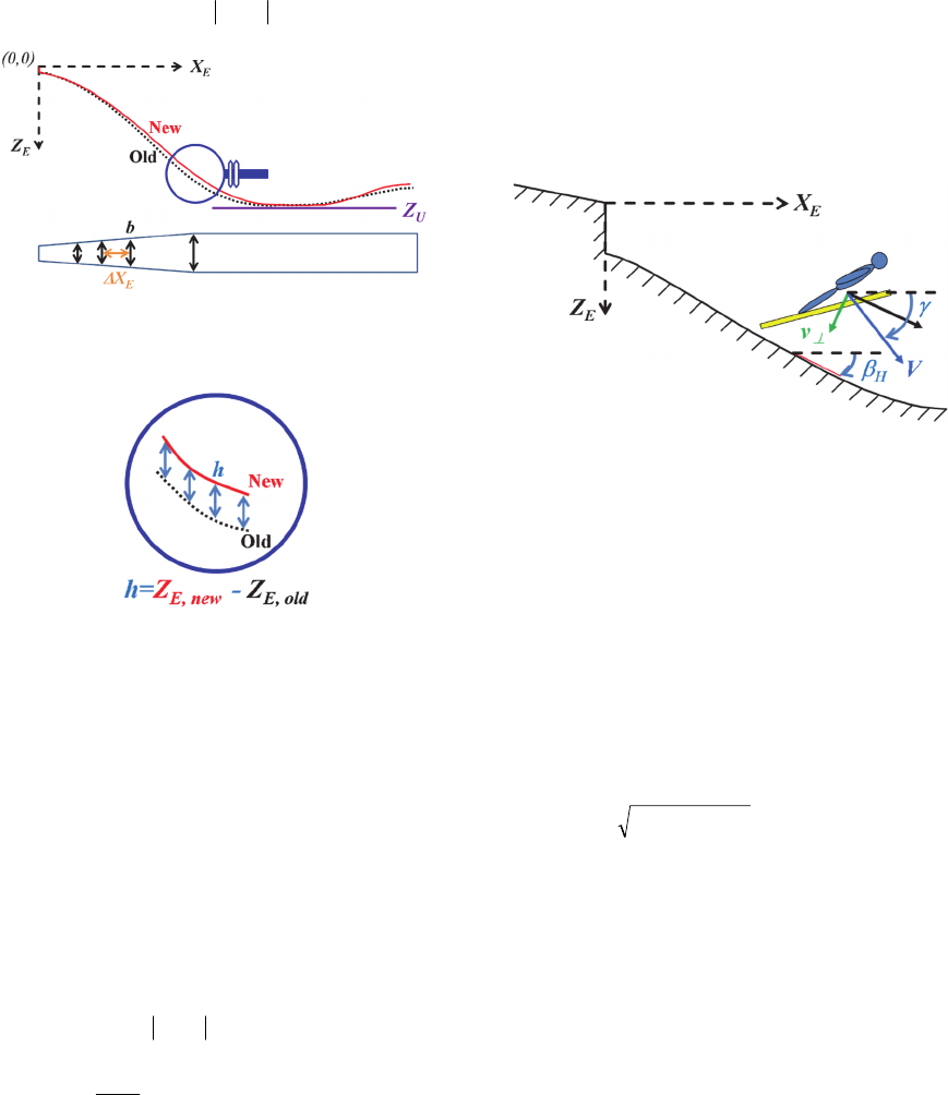
1. The origin is defined as being at the edge of the
take-off table, while the X
E
-axis is in the horizontal
forward direction and the Z
E
-axis is vertically
downward. The height difference between the old
Zao and the new Zao at X
E
is denoted by h(X
E
) as
shown in Figure 2. The width at X
E
is denoted by
b(X
E
). The amount of material needed to construct
the new jumping hill is derived using equation (1).



132
0
:
EEE
dXXbXhmaterialofAmount
(1)
Figure 1: Inertial coordinate system.
The landing profiles of the old and the new Zao.
Figure 2: Height difference between the old and the new
Zao.
The construction fee depends on the height to
which material needs to be taken to construct the
new hill. The greater the height, the more expensive
the construction fee. Here, the lowest cost is at Z
U
(at
the bottom of the slope) and this is assumed to be
200 Japanese yen per 1 m
3
, while the highest cost is
at Z
E
=0 (at the top of the slope), which is assumed to
be 10,000 yen per 1 m
3
on the basis of experience.
The cost between Z
U
and Z
E
=0 is derived using a
linear relationship between cost and height.
Therefore, the construction fee, F1, can be estimated
using equation (2).



132
0
1
EE
XbXhF
(2)
2.2 Safety Landing
The safety on landing was estimated on the basis of
the landing velocity (McNeil et al., 2012). In order
to estimate the landing velocity, the flight trajectory
needs to be simulated. This is discussed in section 3.
The landing velocity is the velocity component
perpendicular to the landing slope at the instance of
landing (Figure 3), and this needs to be small to
reduce the impact and make the landing safer. The
landing velocity, F2, is shown in equation (3), where
the flight path angle and the slope of the landing hill
at the landing point are denoted by γ and β
H
.

H
VvF  

sin2
(3)
Figure 3: Landing velocity, v
┴
.
2.3 Flight Distance
A ski jumping hill should be designed so that it
contributes to the creation of an exciting spectacle,
which means that the jumpers have longer flight
distances. The flight distance is defined by the
distance along the profile of the landing slope. F3,
which is the flight distance multiplied by -1, is
obtained from equation (4). The flight trajectory
needs to be simulated in order to determine the
landing point, X
E
(tf). Here, the flight time is denoted
by tf. This is discussed in section 3.




E
tfX
newEE
dXZXF
E


0
2
,
2
3
(4)
2.4 Difficulty for Unskilled Jumpers
(Variation in the Flight Distance)
The landing slope in Zao is designed to be a difficult
slope for unskilled jumpers. The flight distances of
unskilled jumpers are less than those of skilled
jumpers because they are unable to satisfy the
optimal conditions from take-off through to landing.
Therefore, a landing slope for which the variance in
the flight distance is large is defined as a difficult
slope for unskilled jumpers.

EUEE
U
dXZXZ
Z






 200
9800
Optimizing the Design of the Landing Slope of the Zao Jumping Hill
209

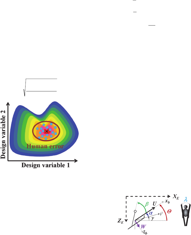
The variance in the flight distance multiplied by -
1, F4, is defined by equation (5), where FD
L
is the
local longest flight distance, shown by × in Figure
4, FD
i
are simulated flight distances around FD
L
,
shown by ● , and n is the number of flight
simulations. The abscissa and the ordinate in Figure
4 are design variables, which are the angles given in
#7 through #22 in Table 1. The ellipse in Figure 4
corresponds to the human error.Since the jumper is
not a robot, there will be some human error, which
shortens the flight distance. The human error is
assumed to be 2° for all angles from #7 through #22.
Fifty Monte-Carlo simulations (i.e. n=50) were
carried out to estimate F4.

1
4
1
2





n
FDFD
F
n
i
Li
(5)
Figure 4: Contour map of flight distance.
FD
L
: Longest flight distance shown by ×,
FD
i
: Flight distances around FD
L
shown by ●.
3 FLIGHT SIMUULATION
In order to estimate F2, F3 and F4, the flight
trajectory needs to be simulated. It is assumed that
the motion of the body–ski combination occurs in a
fixed vertical plane. The coordinate system for the
body is shown in Figure 5. The origin is defined as
the center of gravity of the body–ski combination.
In terms of coordinate transformations (Stevens
and Lewis, 2003) we then have
 sincos WUX
E

(6)
 cossin WUZ
E

(7)
Here, (U, W) are the (x
b
, z
b
) components of the
velocity vector. The equations of motion and the
moment equation are
 QWmgX
m
U
a
 sin
1

(8)
 QUmgZ
m
W
a
 cos
1

(9)
yy
a
I
M
Q 

(10)
Q

(11)
Here, (X
a
, Z
a
) are the (x
b
, z
b
) components of the
aerodynamic force, Q is the y
b
component of the
angular velocity vector, m is the mass of the body–
ski combination, g is the gravitational acceleration,
M
a
is the y
b
component of the aerodynamic moment,
and I
yy
is the moment of inertia of the body–ski
combination on the y
b
-axis. The flight trajectory
(X
E
(t), Y
E
(t), Z
E
(t)) can be obtained by integrating
Equations (6) through (11) numerically.
The aerodynamic forces X
a
and Z
a
in Equations
(8) and (9) are derived from D and L as given in
Eqns. (12) and (13).
 cossin DLX
a

(12)
 sincos DLZ
a

(13)
The aerodynamic drag and lift and moment in Eqns.
(10), (12) and (13) were all obtained during wind
tunnel tests as functions of α, β and λ (Seo,
Watanabe and Murakami, 2004). The wind tunnel
data were acquired for α at 5° intervals between 0°
and 40°, and for β at intervals of 10° between 0° and
40°. The ski-opening angle λ was set at either 0°,
10° or 25°. The torso and legs of the model were
always set in a straight line. The tails of the skis
were always in contact on the inner edges.
Figure 5: Coordinate system for the body and definition of
characteristic parameters.
4 DESIGN VARIABLES
The 22 design variables are shown in Table 1. The
first six are concerned with the landing slope (Figure
6), while the other 16 are concerned with various
angles of the jumper during the jump. The time
variations of β and λ are estimated on the basis of
icSPORTS 2015 - International Congress on Sport Sciences Research and Technology Support
210

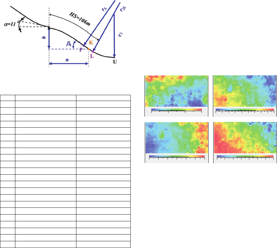
the spline curves, which are constructed from the
control points, #9 through 22, in Table 1. The take-
off table is at an angle of 11 degrees downhill and
the hill size (HS) is set at 106 meters, following a
request from Yamagata city hall. The mass of the
body-ski combination is assumed to be 50 kg, the
take-off speed along and perpendicular to the take-
off table are assumed to be 24.55 m/s and 2 m/s,
respectively.
Optimization was carried out with the aid of a
genetic algorithm (GA). The ‘ranges for GA’, which
are also shown in Table 1, are defined such that they
cover practical values.
In the optimization process, all the objective
functions, from F1 through F4, should be
minimized. The optimization is to determine which
set of design variables makes all the objective
functions smallest.
Figure 6: Landing slope and design variables.
Table 1: Design variables.
# Design variables Ranges for GA
1 n
70～90 m
2 β
k
30～35 °
3 r
L
200～240 m
4 r
2
80～100 m
5 r
2L
80～100 m
6 h/n
0.541～0.543
7 Θ
0
-11～10 °
8 Q
0
-40～10 °/s
9 β at 0.3sec.
20～38 °
10 β at 1.3sec.
2～38 °
11 β at 2.3sec.
2～38 °
12 β at 3.3sec.
2～38 °
13 β at 4.3sec.
2～38 °
14 β at 5.3sec.
2～38 °
15 β at 6.3sec.
2～38 °
16 λ at 0.3sec.
2～28 °
17 λ at 1.3sec.
2～28 °
18 λ at 2.3sec.
2～28 °
19 λ at 3.3sec.
2～28 °
20 λ at 4.3sec.
2～28 °
21 λ at 5.3sec.
2～28 °
22 λ at 6.3sec.
2～28 °
5 CONSTRAINTS
Due to financial reasons, the amount of material
needed to reconstruct the Zao jumping hill was
limited to
 less than 1.0 meters at X
E
=45
 less than 2.0 meters at X
E
=80
 less than 2.0 meters at X
E
=131.9 (old U point)
Moreover, α,β and λ (Figure 5) were limited by the
experimental ranges, as follows.
 0
° < α <40 °
 0
° <β<40 °
 0
° <λ<30 °
Finally, only flight distances of more than 84 meters
were considered.
6 RESULTS AND DISCUSSIONS
Self-organizing maps (SOM) of the objective
functions are shown in Figure 7. These are contour
maps colored by each objective function value. Blue
denotes the lowest value, while red denotes the
highest. A SOM is useful for enabling low-
dimensional views of high-dimensional data
(Kohonen, 1995).
7-a: F1, Construction fee 7-b: F2, Safety on landing
7-c: F3, Flight distance
7-d: F4, Variation in flight
distance
Figure 7: Self-organizing maps of the objective functions.
It can be seen from Figures 7-b and 7-d that the
color patterns of the contour maps are almost same.
Therefore, it can be concluded that the safety on
landing (F2) is almost equivalent to the difficulty for
unskilled jumpers (variation in flight distance, F4).
The safest landing is where the gradient of the
landing slope at the landing point is almost parallel
to that of the flight trajectory of the jumper. On the
3197696 4542456 5887216 7231976
1.0 1.8 2.6 3.4 4.2 4.9 5.7 6.5 7.3 8.1
-113 -108 -104 -99 -95 -90 -86
-9.1 -8.0 -6.9 -5.8 -4.7 -3.6 -2.5 -1.4
Optimizing the Design of the Landing Slope of the Zao Jumping Hill
211

other hand, the same gradient for the flight trajectory
and the landing slope at the instance of landing gives
a larger variation in flight distance. This is the
reason why the safety on landing (F2) is almost
equivalent to the difficulty for unskilled jumpers
(F4).
On the other hand, the contour maps of Figures
7-b and 7-d are almost the converse of that in Figure
7-c. This means that there is a trade-off between the
flight distance (Figure 7-c) and the other two
objective functions (Figures 7-b & 7-d). Although
the lowest values for all the objective functions
gives the ideal situation, it is impossible to meet this
criterion. This is because the four objective
functions conflict with one another. The extreme
case of the longest flight distance is located at the
bottom left hand side of the SOM, where Figure 7-c
shows the lowest value and Figures 7-b and 7-d
show almost their highest values. The landing slope
that produces the longest flight distance gives the
worst safety on landing (dangerous landing) and is
the most difficult for unskilled jumpers (the
difference in flight distance between skilled and
unskilled jumpers is small).
The contour map of Figure 7-a is completely
different from the other three maps (Figure 7-b, 7-c
& 7-d). The color gradient of Figure 7-a is in the
transverse direction, while the color gradients of the
other three maps are in the lateral direction.
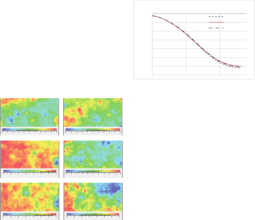
8-a: dv1, n 8-b: dv2, β
k
8-c: dv3, r
L
8-d: dv4, r
2
8-e: dv5, r
2L
8-f: dv6, h/n
Figure 8: Self-organizing maps of design variables
concerned with the landing slope.
Self-organizing maps for the 6 design variables
concerned with the landing slope are shown in
Figure 8. It can be seen that the color pattern of
Figure 8-f is almost the same as those of Figures 7-b
and 7-d, while it is almost the converse of that in
Figure 7-c. This means that the three objective
functions, F2, F3 and F4 are influenced by h/n. It is
self-evident that the smaller h/n makes the flight
distance shorter, and vice versa.
The color gradient of Figure 8-a, n, is in the
transverse direction, as in Figure 7-a. This means
that F1 is influenced by n.
The color patterns of the other four design
variables in Figure 8 do not match those in Figure 7.
Therefore, these four design variables, β
k
, r
L
, r
2
, r
2L
,
do not affect the objective functions.
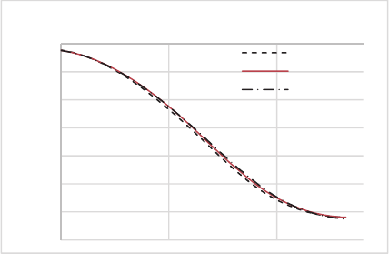
Figure 9: Comparison between the old Zao landing slope
and two examples.
Extreme examples of landing slopes are shown
in Figure 9. The broken line shows the profile of the
old Zao landing slope, the solid line shows the
profile of the lowest cost landing slope (optF1) and
the dash-dot line shows the profile which produces
the safest landing (optF2). It is possible to control
the construction fee, the flight distance and so on, by
changing the profile of the landing slope. The profile
of the low cost slope coincides with the old profile
especially at greater height (around Z
E
=10), though
the profile is different at lower levels (around
Z
E
=50).
On the other hand, the slope with the safest
landing (optF2) is steeper around X
E
=70. This
steeper slope tends to coincide with the flight
trajectory. Therefore, the velocity component
perpendicular to the landing slope is small. The solid
line (optF1) comes close to the dash-dot line (optF2)
at around X
E
=70.
Other, more extreme, examples of landing slopes are
shown in Figure 10. The profile which produces the
longest flight distances (optF3) is almost the same as
that of the most difficult case (optF4) at X
E
=40,
while it is lower at X
E
=80. Since the flight distance
76 76 77 78 79 80 80 81 82 83 83 31 32 32 32 33 33 33 33 34 34 34
207 212 216 221 225 230 235 239 87 88 89 90 91 92 94 95 96 97 98
92 93 95 96 97 98 99 100 0.54 0.54 0.54 0.54 0.54 0.54 0.54 0.54
0
10
20
30
40
50
60
70
050100
ZE [m]
XE [m]
OldZao
optF1
optF2
icSPORTS 2015 - International Congress on Sport Sciences Research and Technology Support
212

is defined by the distance along the profile, as given
by equation (4), the profile of the solid line produces
longer flight distances for the same trajectory.
Figure 10: Comparison between the old Zao landing slope
and two examples.
7 CONCLUDING REMARKS
Optimization of the design of the landing slope was
carried out. The content of the paper is summarized
as follows:
 Four objective functions, which are the
construction fee, the safety on landing, the flight
distance and the difficulty for unskilled jumpers,
were considered.
 It is possible to control the four objective
functions by changing the profile of the landing
slope.
 Safety on landing is almost equivalent to the
difficulty for unskilled jumpers (variation of
flight distance around the local longest flight
distance).
 There is a trade-off between long flight distance
and the safety on landing and the difficulty for
unskilled jumpers.
 The construction fee is influenced by n (the
horizontal distance between the edge of the take-
off table and the K-point).
 The safety on landing, the flight distance and the
difficulty for unskilled jumpers are influenced by
h/n, the ratio of the height difference and the
horizontal distance between the edge of the take-
off table and the K-point.
ACKNOWLEDGEMENTS
This work is supported by a Grant-in-Aid for
Scientific Research (A), No. 15H01824, Japan
Society for the Promotion of Science.
REFERENCES
Kohonen T., 1995. Self-Organizing Maps, Springer,
Berlin, Heidelberg.
McNeil A. J., Hubbard M. and Swedberg, A. D., 2012.
Designing tomorrow’s snow park jump, Sports
Engineering, 15, 1-20
Stevens B. and Lewis F., 2003. Aircraft control and
simulation, Wiley, Hoboken, New Jersey, 2
nd
edition.
Seo K., Watanabe I. and Murakami M., 2004.
Aerodynamic force data for a V-style ski jumping
flight. Sports Engineering, 7, 31-39.
0
10
20
30
40
50
60
70
050100
ZE [m]
XE [m]
OldZao
optF3
optF4
Optimizing the Design of the Landing Slope of the Zao Jumping Hill
213