Using the Cluster-based Tree Structure of k-Nearest Neighbor to Reduce

the Effort Required to Classify Unlabeled Large Datasets

Elias de Oliveira

, Howard Roatti

, Matheus de Araujo Nogueira

, Henrique Gomes Basoni

and Patrick Marques Ciarelli

Programa de P´os-Graduac¸ ˜ao em Inform´atica, Universidade Federal do Esp´ırito Santo,

Av. Fernando Ferrari, 514, Goiabeiras Vit´oria, ES 29075-910, Brazil

Programa de P´os-Graduac¸˜ao em Engenharia El´etrica, Universidade Federal do Esp´ırito Santo,

Av. Fernando Ferrari, 514, Goiabeiras Vit´oria, ES 29075-910, Brazil

Fundac¸˜ao de Assistˆencia e Educac¸˜ao FAESA, Av. Vit´oria, 2.220 - Monte Belo, 29053-360 Vit´oria, ES, Brazil

Keywords:

Text Classiﬁcation, Social Network, Textmining.

Abstract:

The usual practice in the classiﬁcation problem is to create a set of labeled data for training and then use it to

tune a classiﬁer for predicting the classes of the remaining items in the dataset. However, labeled data demand

great human effort, and classiﬁcation by specialists is normally expensive and consumes a large amount of

time. In this paper, we discuss how we can beneﬁt from a cluster-based tree kNN structure to quickly build

a training dataset from scratch. We evaluated the proposed method on some classiﬁcation datasets, and the

results are promising because we reduced the amount of labeling work by the specialists to 4% of the number

of documents in the evaluated datasets. Furthermore, we achieved an average accuracy of 72.19% on tested

datasets, versus 77.12% when using 90% of the dataset for training.

1 INTRODUCTION

The problem of data classiﬁcation is pervasive, and

its importance increases in many ways as the amount

of available data abounds. For instance, the volume

of publicly available video, audio and text, as some

simple forms of data, is steadily growing in many free

reservoirs.

The common way of dealing with the data orga-

nization problem is to have a set of labeled data for

training and then to use this portion of data to pre-

dict the classes for the remaining items of the data

set (Baeza-Yates and Ribeiro-Neto, 2011). However,

the creation of this labeled subset of data is costly

and time-consuming (Cai et al., 2013). In some real-

world situations, data arrive on a streaming basis, and

experts are asked to organize it on the ﬂy for their

current needs and interests. Therefore, a tool to help

them semantically group the data according to their

organization design while simultaneously minimizing

their effort in carrying out this task is needed (Saito

et al., 2014; Costa et al., 2013; Cai et al., 2013; Hoi

et al., 2009).

This problem is frequent in areas such as social

media (Lo et al., 2015), librarianship (Li et al., 2007),

document organization (Malo et al., 2011), and eco-

nomic activity classiﬁcation (Ciarelli et al., 2009). In

particular, social media have recently presented us

with many users’ information worthwhile for market

analysis, event planning, and product monitoring. For

instance, Twitter is one of the most popular social net-

works (Portal, 2015). To capture data from Twitter,

the most common approach is to collect a number of

tweets from Twitter’s Application Programming In-

terface (API) based on some given keywords or previ-

ously known hashtags (Bruns and Liang, 2012; Gun-

decha and Liu, 2012). We chose the hashtags, or key-

words, that encompass the subjects in which we are

interested in studying. Nevertheless, using only these

tools to ﬁnd and understand the messages conveyed

by the goal masses is not sufﬁcient due to hashtag hi-

jacking actions (Hadgu et al., 2013), the variety of

viewpoints within a community, and other problems.

Hence, conventional subject text classiﬁcation plays

an important role in organizing this type of short doc-

ument. In fact, the huge number of small documents

to be organized into subjects challenges the resources

and techniques that have previously been used (Se-

bastiani, 2002; Berry, 2003).

In the case of one who is listening to what people

Oliveira, E., Roatti, H., Nogueira, M., Basoni, H. and Ciarelli, P..

Using the Cluster-based Tree Structure of k-Nearest Neighbor to Reduce the Effort Required to Classify Unlabeled Large Datasets.

In Proceedings of the 7th International Joint Conference on Knowledge Discovery, Knowledge Engineering and Knowledge Management (IC3K 2015) - Volume 1: KDIR, pages 567-576

ISBN: 978-989-758-158-8

567

are saying through a social network channel, the anal-

ysis starts just after totally or partially collecting the

data (Oliveira et al., 2014). This is the point at which

the experts start to design the classes of messages that

they want to study and the messages that will be left

out because they are irrelevant to intended audience.

In this paper, we discuss an approach for the situ-

ation in which we do not have a training dataset from

the start. This is a common situation when addressing

social media streaming data but is not exclusiveto that

scenario. To prepare the data for the supervised classi-

ﬁcation procedure, our approach ﬁrst creates a hierar-

chy structure from a cluster-based sequence by asking

the expert to label some documents in each formed

cluster.

The strategy applied here is similar but superior

to that proposed by Oliveira et al. (2014). Here,

we direct the formation of each cluster to conform

to the structure of the tree proposed by Zhang and

Srihari (2004). As a consequence, a) we are able

to build a very small training dataset from scratch,

which is less than 4% on average of the total datasets;

b) we can achieve an average level of accuracy bet-

ter than 71.65%, versus 77.12%, when using 90% of

the dataset for training; and c) with our approach, the

testing time decreases by an average order of 10.

This work is organized as follows. We present the

general problem and its context in Section 2. In Sec-

tion 3, some related works are brieﬂy reviewed. In-

spired by the work presented by Zhang and Srihari

(2004), in Section 4, we describe the structure used

for building our training dataset to save user work-

load and improve the overall quality of classiﬁcation

metrics. In Section 5, we describe the methods and

results of the experiments. Conclusions are presented

in Section 7.

2 THE PROBLEM DESCRIPTION

The number of tweets, instant messages, photos,

videos and other forms of communication that are

transmitted in social media is large. The volume of

data to be processed by analysts of information is thus

a great challenge (Bastos et al., 2015).

In events such as those in which a multitude of

people are constantly expressing their opinions, in-

tentions and dislikes (Wolfsfeld et al., 2013; Bastos

et al., 2012), analysts have difﬁculty in organizing

all of the conveyed information into themes of in-

terest. Oliveira et al. (2014) reported on a typical

analysis performed on the Brazilian national discus-

sion regarding the Marco Civil on the Internet. The

dataset was formed from the exchange of ordinary

people’s messages through Twitter channels tagged

by the hashtag

#MarcoCivil

and

@MarcoCivil

. The

data were collected in the period from August 2012

to December 2013. In addition to hashtags, the au-

thors sought the twitter data stream using the keyword

"marco civil"

and any hashtag that contained the

sub-string

marcocivil

to create a dataset with 2080

tweets that we henceforth call MarcoCivil.

Similarly, in many other disputes of interest, peo-

ple have several opinions about a particular theme.

Therefore, to better address the social problem, the

government and politicians must understand each

class of demands to determine the social consensus.

We claim that the ﬁrst step is to organize the opinions

into classes such that each class can be addressed ac-

cordingly based on their needs and possibilities.

This problem is not at all simple, because each

group of analysts can have their own objectives and

perspectives and can thus label the same opinions

within a dataset differently. We argue that although

one can use predeﬁned classes to classify tweets (Sri-

ram et al., 2010), such strategies are not always ac-

curate with regard to the user’s needs. Moreover,

the great volume of data to be processed demands

improvements in conventional methods for machine

learning techniques so that they should incrementally

adjust themselves according to users’ needs.

In this work, we propose the use of a methodology

that reduces human effort and optimizes the computa-

tional cost of an automatic classiﬁcation system when

performing data organization in groups.

3 RELATED WORKS

Currently, the large amount of data to be analyzed,

categorized and organized makes it increasingly un-

feasible to use manual procedures to process it with

sufﬁcient speed. To overcome this problem, an in-

creasingly common approach is to use supervised ma-

chine learning techniques to assist humans in process-

ing large datasets. A signiﬁcant advantage of this ap-

proach is that a task can be completed quickly, contin-

uously and uninterruptedly. The literature has shown

that this approach is effectivein many areas (Lin et al.,

2012; Cruz and Wishart, 2007; Blanzieri and Bryl,

2008).

However, supervised machine learning techniques

achieve relevant results only when they are trained

with datasets that were properly labeled by experts.

The great problem is that labeled datasets are not al-

ways available, or that the amount of labeled data may

be quite limited. Moreover, in many situations, it is

not easy to obtain labeled data because the task of cat-

SSTM 2015 - Special Session on Text Mining

568

egorizing data is expensive, is time consuming, must

be performed by experts, and involves subjectivity

(people may place the same sample in different cat-

egories). Further, some experts do not collaborate be-

cause they are afraid of being replaced by machines.

Some attempts to facilitate the task of labeling

large datasets have been proposed in the literature.

One of the methods explored by some researchers

(Vens et al., 2013; Duarte et al., 2013; Zeng et al.,

2003) is based on clustering, which is anunsupervised

method in which the experts label only a small dataset

(usually selected by algorithms). Using these data, the

method labels the remaining unseen data based on the

groups created by the previous clustering procedure.

Among the supervised approaches, the kNN al-

gorithm (Cover and Hart, 1968) has been extensively

used as a powerful non-parametric technique for pat-

tern recognition. The easy implementation and the

relevant results of kNN have encouraged many re-

searchers to use it as one of the ﬁrst algorithms to

treat a classiﬁcation task. Moreover, the fact that it

has only one parameter to be adjusted makes it easy

to ﬁne-tune to a variety of situations. However, it re-

quires intensive dissimilarity computations and mem-

ory usage, mainly for large training sets. In many ap-

plications, the computational cost of ﬁnding the near-

est neighbors imposes practical limits on the training

set size and the acceptable time to return an output.

Therefore, speeding up the kNN search is an essential

step to make kNN more useful in the classiﬁcation of

huge datasets.

Algorithms for speeding up the kNN search em-

ploy one or more criteria to avoid using all of the sam-

ples in an available training set when trying to ﬁnd

probable labels of a new unclassiﬁed pattern. These

algorithms can fall into one of two categories (Zhang

and Srihari, 2004): template condensation and tem-

plate reorganization. Template condensation removes

redundant patterns, such that the training set size is re-

duced and the search is made faster (Angiulli, 2007,

2005). The second category includes those that re-

organize good patterns for a training set such that

the kNN search can be more efﬁcient (Kim and Park,

1986). A third category is a hybrid of template con-

densation and template reorganization (Brown,1995).

In this work, we use an algorithm of template re-

organization proposed by Zhang and Srihari (2004)

because this type of algorithm is more efﬁcient than

template condensation algorithms are.

To sum up, we propose an approach with two steps

to perform the categorization of some large datasets.

In the ﬁrst step, a procedure is used to cluster the

datasets, and some speciﬁc samples are selected to

be categorized by experts. This procedure automat-

ically labels the samples in the most trivial cases of

clustering. Nevertheless, it is possible that not all of

the samples will be labeled at this stage. Then, the

next step is conducted, in which the data labeled in

the previous step are used to train a kNN algorithm,

such that it can be employed to classify the remaining

data.

In the next section, we show some of the results

of our strategy applied over some well-known litera-

ture datasets. We discuss the results with and with-

out the use of the clustering phase, and later with the

clustering phase as a process to form a training set

for the following classiﬁcation phase using the con-

ventional kNN and cluster-based tree kNN (kNN++)

algorithms.

4 THE ALGORITHM

Unlike Zhang and Srihari (2004), we address the

problem of text classiﬁcation from the point at which

we do not yet have a labeled dataset. Therefore,

we preprocess our entire dataset to form this training

data. Only then do we follow the idea proposed by

Zhang and Srihari (2004).

4.1 Building the Training Dataset

Initially, we consider D to be the whole dataset of

|D| documents. The ﬁrst step is to cluster the whole

dataset into Ω = {S

,...,S

}, S

⊂ D, where i =

1,2,... , p. We start this process either by ﬁxing the

number p of clusters to be formed or by arbitrarily

choosing a value for ρ, which is the average internal

similarities of documents within each cluster. Note

that every document d

∈ S

is preprocessed and rep-

resented by a vector space of features.

Hence, each d

is a vector such that d

,...,x

) is composed of a set of |d

| terms

and the variable x

≥ 0 (q = 1,2,3, .. .,|d

|) repre-

sents the weight of the term t

in the vector d

. For

the Marco Civil dataset, (described ahead in Section

5) these variables were formed by the product of term

frequency and inverse document frequency (Baeza-

Yates and Ribeiro-Neto, 2011). The other datasets are

already represented in vector space model.

At this point, each S

= {. .. ,d

,..., d

} is a sub-

set of the samples contained in the dataset. Subse-

quently, we sort the members of each S set such that

,..., d

t−2

t−1

= d

} are in increasing or-

der of dissimilarities. Then, we start a process in

which experts are asked to assign labels to some items

of each S

⊂ D until they feel satisﬁed with the ho-

mogeneous characteristics within each of the clusters.

Using the Cluster-based Tree Structure of k-Nearest Neighbor to Reduce the Effort Required to Classify Unlabeled Large Datasets

569

A dissimilarity measure d(.,.) is used to choose the

most dissimilar member of each S

⊂ D cluster. In

this paper, we use the cosine measure for the experi-

ments.

When the experts assign the same label to both of

the most dissimilar members of a cluster d

and d

for instance, we assume that the whole cluster is sim-

ilarly labeled with the previously given label. This

is called labeling by level 0 of the decision (LD

Even when given the same label for both of the far-

thest documents, we may further ask the experts to

check whether d

t−1

still receives the same label. This

is called labeling by level 1 of the decision (LD

This is a narrower level of decision than the previous

one. Similarly, if the pair of labels given at this level

are the same, we assume that the whole cluster must

be labeled with the previously given labels.

Whenever the most dissimilar members of a clus-

ter S

are not assigned the same label by the ex-

perts, we conclude that the documents grouped into

this cluster must be left out of the training set. This

decision can be made at any level of LD

, where

i = 1,2,. .. ,|S

|. The pseudo algorithm is illustrated

by the Algorithm 1.

Algorithm 1: The training dataset building algorithm.

1: procedure CLUSTER(D) ⊲ Ω = {S

,..., S

}

2: Sort each S

⊂ D

3: result: S

= {d

,..., d

t−1

}

4: for l ← 1

p do

Ask the experts to assign

labels for

∈ S

7: if

labels are identical

then

set

∀d

∈ S

the same label

9: else

10:

set

Ω = Ω\S

11: end if

12: end for

13: end procedure

At the end of this process, we will have m = |Ω|

documents, which will be used as templates for the

bottom level B of the cluster-based tree structure pro-

posed by Zhang and Srihari (2004) (see Section 4.2).

4.2 Cluster-based Tree Generation

The cluster-based tree kNN proposed by Zhang

and Srihari (2004) is based on hierarchical class-

conditional clustering over |Ω| samples. In this work,

we build the bottom level B by using the samples la-

beled in the previous section. Another level, called

hyperlevel H , is generated by pulling up one of the

most dissimilar members, d

, for instance, of each

∈ Ω at the end of the procedure described in Sec-

tion 4.1. These members are removed from the bot-

tom level B.

Thus, the properties of each sample d are com-

puted: a) γ(d), the dissimilarity between d and its

nearest neighbor with a different class label; b) ψ(d),

a set of all neighbors that have the same class label as

d and are less than γ(d) away from d; and c) ℓ(d), the

size of the set ψ(d).

Therefore, our cluster tree is built as follows

(Zhang and Srihari, 2004):

Step 1. Initialize the bottom level of the cluster tree

with all template documents that are labeled

during the process described in Section 4.1.

These templates constitute a single level B;

Step 2. ∀S

∈ Ω, extract one of the most dissimilar

samples, for instance d

, and compute the lo-

cal properties of each sample d

= d: γ(d),

ψ(d) and ℓ(d). Then, rank all clusters S

descending order of ℓ(.);

Step 3. Take the sample d

with the biggest ℓ(.) as

a hypernode, and let all samples of ψ(d

) be

nodes at the bottom level of the tree, B. Then,

remove d

and all samples in ψ(d

) from the

original dataset, and set up a link between d

and each pattern of ψ(d

) in B;

Step 4. Repeat Step 2 and Step 3 until the Ω set be-

comes empty. At this point, the cluster tree is

conﬁgured with a hyperlevel, H , and a bot-

tom level, B;

Step 5. Select a threshold η and cluster all templates

in H so that the radius of each cluster is less

than or equal to η. All cluster centers form

another level of the cluster tree, P ;

Step 6. Increase the threshold η and repeat Step 5 for

all nodes at the level P until a single node is

left in the resulting level.

At the level of hyperlevel H , all samples that are

connected belong to the same class. The levels above

are based on nearness among a set of nodes such that

samples of different classes can be grouped. The η

value is critical for generating a cluster tree; more-

over, its value must be increased as a function of the

number of iterations in Step 5. A simple solution

proposed by Zhang and Srihari (2004) is to compute

η(i) = µ

− α

1+i

, where α is a constant and µ

and σ

are the mean and standard deviation of the dissimilar-

ities between the nodes at iteration i, respectively.

In the next section, we show how to use this tree

to classify an unseen document into its most probable

class.

SSTM 2015 - Special Session on Text Mining

570

4.3 The Classiﬁcation Test

After building the cluster tree, the next procedure is

to classify an unseen sample x. This procedure is per-

formed as follows (Zhang and Srihari, 2004):

Step 1. First, we compute the dissimilarity between x

and each node at the top level of the cluster

tree and choose the ς nearest nodes as a node

set L

;

Step 2. Compute the dissimilarity between x and

each subnode linked to the nodes in L

, and

again choose the ς nearest nodes, which are

used to update the node set L

;

Step 3. Repeat Step 2 until reaching the hyperlevel

in the tree. When the searching stops at the

hyperlevel, L

consists of ς hypernodes;

Step 4. Search L

for the hypernode: L

{Y|d(y,x) ≤ γ(d),y ∈ L

}. If all nodes in L

have the same class label, then this class is as-

sociated with x and the classiﬁcation process

stops; otherwise, go to Step 5;

Step 5. Compute the dissimilarity between x and ev-

ery subnode linked to the nodes in L

, and

choose the k nearest samples. Then, take a

majority voting among the k nearest samples

to determine the class label for x.

At the level of hyperlevel,the class of a given sam-

ple x is decided only if all clusters (the elements in L

)

into which x falls have the same class level. The larger

the value of ς is, the higher the accuracy of recogni-

tion will be; however, the computational cost is also

higher.

5 EXPERIMENTS AND RESULTS

Our proposed method was evaluated using Iris and

TAE, which are available and described in detail at the

UCI Machine Learning Repository (Newman et al.,

1998)

; Reuters8, Reuters52, and WEBKB-4 avail-

able from Cardoso-Cachopo (2007); and the Marco

Civil dataset collected from Twitter, which was kindly

shared with us by its owners (Oliveira et al., 2014).

This latter dataset was classiﬁed using two distinct

groups of classes, so it was analyzed as two datasets:

Marco Civil I (MC-I) and Marco Civil II (MC-II).

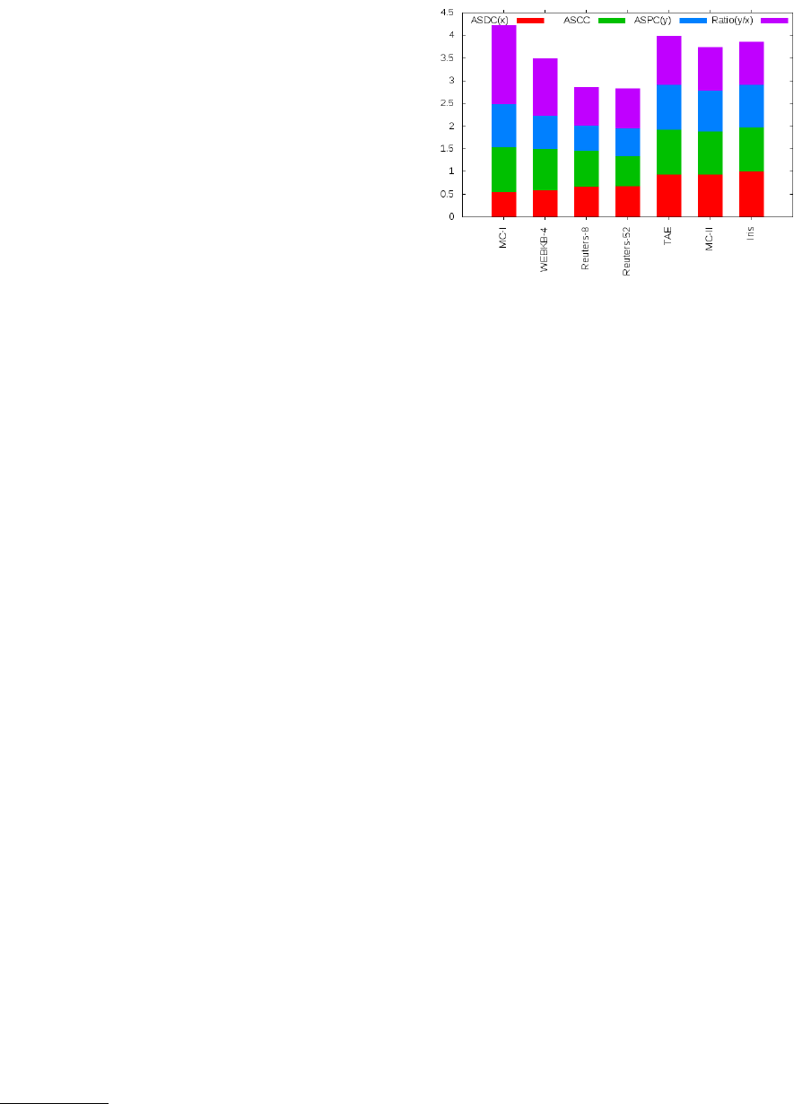
Figure 1 graphically represents the numbers that

describe the datasets. We ordered the list of datasets

by their ASDC(x), ASCC, ASPC(y) and ratio(y/x).

This ﬁgure shows that the TAE, MC-II and Iris

https://archive.ics.uci.edu/ml/datasets.html

Figure 1: Datasets feature-characterization histogram.

datasets are more similar to one another than to the

rest of the datasets.

In Table 2, we describe each of the datasets. Iris

has the fewest documents, only 150, followed by TAE

with 151 documents. In terms of classes, Reuters52

has the most classes, 52, but does not have the most

features. MC-II has the largest number of features,

4804, followed by MC-I, which also has one of the

smallest numbers of classes, only 3, along with Iris

and TAE.

Table 1 provides the geometric characterization of

the datasets used in this work. ASDC is the Aver-

age Similarity between every Document of a class and

their respective Centroid. On the one hand, the values

in Table 1 show that samples in the same class are

spatially well separated when the value of ASDC is

low. This is found the case of the MC-I samples in

the ﬁrst column of the table. We can say that on aver-

age, classes in MC-I have their items more scattered

but that the items in Iris are the most concentrated,

followed by the items in MC-II.

On the other hand, ASCC is the Average Similar-

ity between the Centroids of Classes and the dataset

main Centroid. We can see that the dataset TAE has

all its classes very close to one another because its

ASCC value is high. An interesting situation is seen

in the MC-I dataset, which follows the TAE dataset

with an ASCC greater than 0.98. This is because its

ASDC has the lowest value; that is, this class is the

one with the most overlapped members.

ASPC is the Average Similarity between Pairs of

Centroids. The high value of ASPC indicates that the

classes are overlapping, thereby causing high rates of

y/x. In Figure 1 we have a different way of looking

at these numbers. Therefore, one can conclude that

the samples of MC-I, WEBKB-4, Reuters8, etc., rep-

resent the most tangled datasets. They have very scat-

tered elements in their classes, but their classes are

very close to each other. We thus claim that these ﬁg-

Using the Cluster-based Tree Structure of k-Nearest Neighbor to Reduce the Effort Required to Classify Unlabeled Large Datasets

571

Table 1: Geometric characterization of the datasets used in the experiments.

Dataset ASDC (x) ASCC ASPC (y) Ratio (y/x)

Iris 0.998877 0.983528 0.936333 0.937385

MC-I 0.553464 0.986026 0.953384 1.722577

MC-II 0.937716 0.952153 0.894900 0.954340

Reuters-52 0.680510 0.676758 0.596804 0.876995

Reuters-8 0.672568 0.790993 0.557013 0.828188

TAE 0.936024 0.997729 0.990932 1.058661

WEBKB-4 0.592095 0.914236 0.734080 1.239801

Table 2: Characterization of the datasets.

Dataset #Doc #Class #Feature

Iris 150 3 4

MC-I 2044 3 4421

MC-II 2109 9 4804

Reuters 52 9100 52 3000

Reuters 8 7674 8 3000

TAE 151 3 5

WEB KB 4 4199 4 3000

ures have a great impact on the classiﬁcation results.

The climax of the discussion on the Marco Civil

for the Internet by the Brazilian parliament occurred

between the end of 2009 and beginning of 2013, when

the parliament was discussing and working on pass-

ing a new law for the country regarding this mat-

ter. The discussions related to this theme were fur-

ther stimulated after the leak of documents by Edward

Snowden, a former employee of the National Secu-

rity Agency, who had obtained unauthorized conﬁ-

dential information about some international govern-

ments from the U.S. government. From that point,

many people started expressing their opinions via

Twitter and other social media channels.

Oliveira et al. (2014) performed the following pre-

processing on the dataset from Twitter. First, iden-

tical tweets and some unreadable data due to some

problems during the collection process were removed

from the dataset.

In the Marco Civil I dataset, the tweets were clas-

siﬁed using the theme of Political Positioning, which

aims to assig a tweet into one of 3 subclasses: Neutral,

Progressive, and Conservative comments. Tweets

which messages are unclear with regard to political

positioning were assigned to the Neutral class. The

messages that were clearly in favor of the broaden-

ing and deepening of the discussions were assigned to

the Progressive class. Finally, the messages that were

against any change of the current legislation were as-

signed to the Conservative class.

In contrast, the Marco Civil II dataset is composed

of tweets that were classiﬁed based on the theme of

Opinion. The goal now is to assign a tweet to one of 9

subclasses: Alert, Antagonism, Support, Compliance,

Explanation, Indignation, Information, Mobilization,

and Note.

Alert is a class that is used to aggregate all tweets

that draw attention to the evolution of the discussion

within the parliament. The Antagonism class gath-

ers the messages in opposition of the approval of the

Marco Civil project. The Support class represents

tweets in favor of both discussion and approval of the

Marco Civil project. Although the Compliance class

has messages showing sympathy towards the project,

they do not show open support to ofﬁcial legislation

of the matter.

Some people posted messages mainly to analyze

and comment on the evolution of the discussions

about the project. These messages were assigned to

the class Note. Although it is very similar to the pre-

vious class, the class Information aims at gathering

tweets that share with the community some sort of

news about the project, not a personal opinion. All

tweets that explain the Marco Civil project, the legis-

lation proposals and their consequences were grouped

within the class Explanation. The Indignation class

included users who are against the news press atti-

tude, the way the deputies postponed the voting in the

parliament, and essentially the lack of any type of leg-

islation about the use of the Internet in Brazil. Finally,

the class Mobilization gathers messages that attempt

to bring people to participation and engagement in the

movement. The following is a tweet that calls on peo-

ple to send a message to their deputies in the Marco

Civil Especial Committee in the parliament:

@idec – Envie uma mensagem agora aos

deputados da Comiss˜ao Especial do Marco

Civil! http://t.co/kslJpTOh

Our focus is on MC-I and MC-II; thus, the other

datasets were also used here to show that our ap-

proach is as suitable as the widely known datasets in

the literature.

SSTM 2015 - Special Session on Text Mining

572

5.1 Analysis of the Results

The ρ value is critical. With a low value of ρ, the

clusters tend to be more homogeneous, but the user’s

workload increases. If the value is high, the number

of clusters is smaller, but they are less homogeneous

(Oliveira et al., 2014). We varied this value in the

range from 0.3 to 0.9. The best value on average was

0.6, which is the chosen value for the experiments re-

ported in this work.

Another important parameter is the value of k for

the kNN implementations. We also tested many val-

ues of k for all kNN algorithms tested in this work:

the conventional kNN (Cover and Hart, 1968; Duda

et al., 2001), the cluster-based tree kNN, and our pro-

posed method, which combines the creation of the

training dataset and the cluster-based tree kNN. Thus,

the value of k that achieved the highest average accu-

racy metric for the Marco Civil datasets was k = 3.

Thus, we arbitrarily chose this value to perform out

our experiments with the rest of the datasets.

Table 3: The algorithm accuracy performance.

kNN++

Data set kNN kNN++ LD

Iris 98.12 92.07 79.71 79.71

MC-I 66.07 64.49 68.92 68.30

MC-II 82.29 81.57 82.80 81.79

Reuters 8 79.79 86.97 77.58 77.09

Reuters 52 96.75 96.90 96.80 96.77

TAE 62.02 60.94 57.31 56.81

WEB KB 4 61.03 64.94 64.57 64.57

77.12 74.77 72.19 71.65

Table 3 shows the results of three different ex-

periments we performed on the datasets. In the ﬁrst

column, we list the datasets used to demonstrate our

claim. In the second column, we show the results of

a version of our conventional kNN algorithm. The

third column, represents our cluster-based tree algo-

rithm. As noted above, we chose k = 3 for all version

of kNN. In addition, all experiments were performed

by applying the 10-fold cross-evaluation; e.g., each

dataset was divided into 10-folds, and each algorithm

was run 10 times, with 9-folds for training and 1 for

testing. A different fold was used as a test each time.

The exception is made in the proposed method, where

we ﬁxed the training set at that sample chosen by the

clustering phase described in Section 4.1 (see also Al-

gorithm 1). Table 3 shows the average results of these

runs.

In general, we may say that the reduction of the

training dataset impacts the quality of the results, as

also reported by Zhang and Srihari (2004). Nonethe-

less, we can see a consistent decay in quality on Iris

and TAE only. This steady decay is also observed

only on the average of the results on the datasets as a

whole.

A different group of results are those in which the

new kNN++ yielded improvements over the conven-

tional kNN. Considering the improvements between

the second and third columns in Table 3, we can see

that these are the cases of Reuters8, Reuters52, and

WEBKB 4.

WEBKB 4 had the minimum quality decay when

it was submitted to the clustering procedure in the

fourth and ﬁfth columns. MC-I and MC-II are the

ones that beneﬁtted the most from the proposed clus-

tering approaches. Both had some deterioration from

kNN to kNN++ but also exhibited some improve-

ments, surpassing the best results with kNN most of

the time.

We can see, from these results, that our proposed

method of creating a training dataset is in fact very

efﬁcient. The results were slightly affected in some

cases, but not much on average. In some cases, the

proposed methodology worked on even boosting the

quality of the results.

Table 4: The algorithm time performance in minutes.

The proposed methods

kNN++

Dataset kNN kNN++ LD

Iris 0.05 1.44 0.56 0.56

MC-I 14.41 9.39 1.28 1.36

MC-II 17.07 4.02 1.03 2.88

Reuters 52 50.79 39.45 3.79 3.88

Reuters 8 42.38 2.57 0.40 0.27

TAE 0.06 0.69 0.18 0.11

WEB KB 4 26.10 1.72 0.40 0.38

21.55 8.47 1.09 1.35

Another dimension of the analysis is to observe

the time performance of the new kNN++ and the

proposed clustering strategy. In Table 4, we show

the time in minutes for the classiﬁcation of only the

test portion of the datasets.To normalize the size of

all datasets, these values refer to the average time to

classify 1000 samples.

In the ﬁrst column of Table 4, we show the

datasets used to conduct the experiments, the sec-

ond column shows the results of the conventional

kNN. This is used for comparison among the other

approaches. We can see in the third column that

the time to classify the same amount of data by the

kNN++ is already inferior to the previous approach.

The speed advantage is 57.02% on average. In the

case of Reuters8, the speed advantage was evenbetter,

achieving a value of 93.93% when classifying 1000

samples.

Using the Cluster-based Tree Structure of k-Nearest Neighbor to Reduce the Effort Required to Classify Unlabeled Large Datasets

573

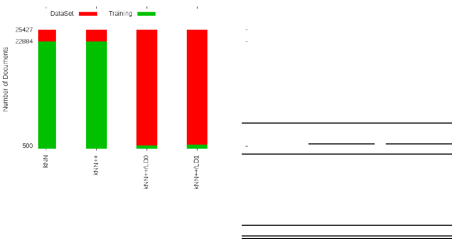
Figure 2: The reduction effort for building the training set.

These time ﬁgures havea further decrease with the

and LD

approaches, which show that our strat-

egy has a good impact on the reduction of the struc-

ture of the algorithm so that it can better classify the

samples.

In addition to the large reduction of classiﬁcation

time and the slight decrease in quality, our approach

provides the users with another advantage, which is

the possibility of forming their training dataset on the

ﬂy with the classiﬁcation of an unlabeled dataset. Fur-

thermore, our strategy drastically reduces the neces-

sary effort for the creation of the training labeled data,

as we can see in Figure 2.

The total number of documents among all datasets

is 25,427. On the one hand, to obtain the results

shown for kNN and the kNN++ in Table 3, we used

9-folds to form the respective training datasets, which

represents than 22,884 documents. On the other hand,

by applying our approach, kNN+ +/LD

{0,1}

, the num-

ber of documents labeled by experts used for train-

ing, totaled 587 for LD

and 778 for LD

. Therefore,

we achieve a reduction to 4% of the previous training

dataset. Note that there is still room for improvement

in our approach.

6 DISCUSSION

The original algorithm proposed by Zhang and Srihari

(2004) includes only one template at the hyperlevel

to represent the set of other documents at the bot-

tom level. In our previous experiments, we used the

∈ S

to play this role (Step 3 in Section 4.2). The

results are shown in Table 3 and Table 4. However, we

noticed during the experiments that a slight modiﬁca-

tion at this point on the original algorithm could bring

even more reduction to the time performance of the

classiﬁcation time. Then, we changed the algorithm

to include not only one of the template to represent the

bottom level documents, but both the most dissimilar

members of the cluster. Therefore, this new version

of the algorithm includes {d

} ∈ S

as member of

the hyperlevel to represent theirs group of documents

at the bottom level.

Table 5: The algorithm accuracy performance.

kNN++ kNN++

Hyperlevel only {d

} with {d

}

Data set LD

Iris 79.71 79.71 84.06 91.30

MC-I 68.92 68.30 63.90 44.70

MC-II 82.80 81.79 80.99 80.83

Reuters 8 77.58 77.09 82.73 82.24

Reuters 52 96.80 96.77 96.72 96.88

TAE 57.31 56.81 63.08 63.08

WEB KB 4 64.57 64.57 64.77 63.90

72.19 71.65 76.61 74.63

As a consequence of this modiﬁcation is that, dur-

ing the classiﬁcation phase, we can now consider also

the information of the second template to decide the

classes that will be assigned to the templates. The re-

sults are shown in Table 5. After the datasets column,

we show in the second and third columns the previous

results when using only {d

} to represent a group of

bottom levels documents. Again, we performed the

experiments using the LD

and LD− 1 strategies, as

explained previously. In the fourth and ﬁfth columns,

we present the results of the modiﬁed algorithm, with

} to represent a group of bottom levels docu-

ments. We can see that the quality of classiﬁcation

for the majority of the datasets improved even further

when comparing to the strategy proposed by Zhang

and Srihari (2004) and nearly reproduced in the sec-

ond and third columns. The worst result was found

for the MC-I. An explanation for such results need a

deeper analysis.

In addition to the quality improvement, this mod-

iﬁcation also reduce even more the classiﬁcation time

performance, as we can see in Table 6. Now, the clas-

siﬁcation can be made more often at the hyperlevel,

so that the algorithm does not need to consume time

processing documents at the bottom level.

7 CONCLUSIONS

In this paper, we proposed a strategy to address the

problem of building a training dataset from scratch for

a text classiﬁcation problem. The goal was to reduce

the human effort required in manual classiﬁcation so

SSTM 2015 - Special Session on Text Mining

574

Table 6: The algorithm time performance in minutes.

kNN++ kNN++

Hyperlevel only {d

} with {d

}

Data set LD

Iris 0.56 0.56 0.00 0.00

MC-I 1.28 1.36 0.22 0.24

MC-II 1.03 2.88 0.33 0.34

Reuters 52 3.79 3.88 1.72 1.85

Reuters 8 0.40 0.27 1.21 1.07

TAE 0.18 0.11 0.00 0.00

WEB KB 4 0.40 0.38 0.49 0.50

1.09 1.35 0.57 0.57

that the manual assignment of labels requires as small

a subset of the dataset as possible. Then, we used this

chosen training dataset to classify the remaining data.

We were inspired by the cluster-based trees kNN

algorithm presented by Zhang and Srihari (2004). We

used their strategy to construct the tree and, at the

same time, chose the items that formed our train-

ing dataset. These chosen items were submitted to

the evaluation of an expert, or experts, for labeling.

Therefore, while choosing these items, we interacted

with the expert to design each node and level of the

tree. At the end, the tree was built with the training

data, and the kNN was ready to be applied to the re-

maining dataset.

The comparison between the results obtained by

our strategy and those produced by an expert in all of

the tested datasets revealed that our approach is able

to imitate the expert up to 72.19% on average, with re-

gard to the accuracy metric while using less than 4%

of the dataset for training. We also applied this tech-

nique to some public datasets and showed that we can

greatly reduce the effort of the expert when construct-

ing the training data without losing much quality in

the classiﬁcation.

We improved the proposed algorithm by Zhang

and Srihari (2004) changing the way the hyperlevel

is built, and the results are promising. We plan to fur-

ther investigate strategies to better form the training

dataset and increase the performance of the proposed

algorithm kNN+ +.

ACKNOWLEDGEMENTS

The ﬁrst author would like to thanks CAPES for its

partial support on this research under the grant n

BEX-6128/12-2.

REFERENCES

Angiulli, F. (2005). FastCondensed Nearest Neighbor Rule.

pages 1–8. IEEE.

Angiulli, F. (2007). Fast Nearest Neighbor Condensation

for Large Data Sets Classiﬁcation. IEEE Transactions

on Knowledge and Data Engineering, 9(11):1450–

1464.

Baeza-Yates, R. and Ribeiro-Neto, B. (2011). Modern In-

formation Retrieval. Addison-Wesley, New York, 2

edition.

Bastos, M., Travitzki, R., and Puschmann, C. (2012). What

Sticks With Whom Twitter Follower-Followee Net-

works and News Classiﬁcation. In Proceedings of In-

ternational AAAI Conference on Weblogs and Social

Media.

Bastos, M. T., Mercea, D., and Charpentier, A. (2015).

Tents, Tweets, and Events: The Interplay Between

Ongoing Protests and Social Media. Journal of Com-

munication, 65(2):320–350.

Berry, M. W. (2003). Survey of Text Mining: Clustering,

Classiﬁcation, and Retrieval. Springer-Verlag, New

York.

Blanzieri, E. and Bryl, A. (2008). A Survey of Learning-

Based Techniques of Email Spam Filtering. Artiﬁcial

Intelligence Review, 29(1):63–92.

Brown, R. L. (1995). Accelerated TemplateMatching Us-

ing Template Trees Grown by Condensation. IEEE

Transactions on Systems, Man and Cybernetics–Part

C: Applications and Reviews, 25(3):523–528.

Bruns, A. and Liang, Y. (2012). Tools and Methods for Cap-

turing Twitter Data During Natural Disasters. First

Monday, 17(4).

Cai, W., Zhang, Y., and Zhou, J. (2013). Maximizing Ex-

pected Model Change for Active Learning in Regres-

sion. In Data Mining (ICDM), 2013 IEEE 13th Inter-

national Conference on, pages 51–60.

Cardoso-Cachopo, A. (2007). Improving Methods for

Single-Label Text Categorization. PhD thesis, Insti-

tuto Superior T´ecnico, Universidade T´ecnica de Lis-

boa. http://ana.cachopo.org/publications.

Ciarelli, P. M., Krohling, A., and Oliveira, E. (2009). Parti-

cle Swarm Optimization Applied to Parameters Learn-

ing of Probabilistic Neural Networks for Classiﬁca-

tion of Economic Activities. I-Tech Education and

Publishing, Viena, Austria.

Costa, J., Silva, C., Antunes, M., and Ribeiro, B. (2013).

Customized Crowds and Active Learning to Im-

prove Classiﬁcation. Expert System and Applications,

40(18):7212–7219.

Cover, T. M. and Hart, P. E. (1968). Nearest Neighbor Pat-

tern Classiﬁcation. IEEE Transactions on Information

Theory, pages 21–27.

Cruz, J. A. and Wishart, D. S. (2007). Applications of Ma-

chine Learning in Cancer Prediction and Prognosis.

Cancer informatics, 2:59–77.

Duarte, J. M. M., Fred, A. L. N., and Duarte, F. J. F. (2013).

A Constraint Acquisition Method for Data Cluster-

ing. Progress in Pattern Recognition, Image Analysis,

Computer Vision, and Applications, pages 108–116.

Using the Cluster-based Tree Structure of k-Nearest Neighbor to Reduce the Effort Required to Classify Unlabeled Large Datasets

575

Duda, R. O., Hart, P. E., and Stork, D. G. (2001). Pattern

Classiﬁcation. Wiley-Interscience, New York, 2 edi-

tion.

Gundecha, P. and Liu, H. (2012). Mining Social Media: A

Brief Introduction. Tutorials in Operations Research,

1(4).

Hadgu, A. T., Garimella, K., and Weber, I. (2013). Po-

litical Hashtag Hijacking in the U.S. In Proceed-

ings of the 22Nd International Conference on World

Wide Web Companion, WWW ’13 Companion, pages

55–56, Republic and Canton of Geneva, Switzerland.

International World Wide Web Conferences Steering

Committee.

Hoi, S., Jin, R., and Lyu, M. (2009). Batch Mode Active

Learning with Applications toText Categorization and

Image Retrieval. IEEE Transactions on Knowledge

and Data Engineering, 21(9):1233–1248.

Kim, B. S. and Park, S. B. (1986). A Fast k Nearest Neigh-

bor Finding Algorithm Based on the Ordered Parti-

tion. IEEE Transactions on Pattern Analysis and Ma-

chine Intelligence, pages 761–766.

Li, X., Chen, H., Zhang, Z., and Li, J. (2007). Automatic

Patent Classiﬁcation using Citation Network Infor-

mation: an Experimental Study in Nanotechnology.

In JCDL ’07: Proceedings of the 2007 Conference

on Digital libraries, pages 419–427, New York, NY,

USA. ACM.

Lin, W.-Y., Hu, Y.-H., and Tsai, C.-F. (2012). Machine

Learning in Financial Crisis Prediction: A Survey.

IEEE Transactions on Systems, Man, and Cybernet-

ics, Part C: Applications and Reviews, 42(4):421–436.

Lo, S. L., Chiong, R., and Cornforth, D. (2015). Using Sup-

port Vector Machine Ensembles for Target Audience

Classiﬁcation on Twitter. Plos One, 10(4):1–20.

Malo, P., Sinha, A., Wallenius, J., and Korhonen, P.

(2011). Concept-Based Document Classiﬁcation Us-

ing Wikipedia and Value Function. Journal of the

American Society for Information Science and Tech-

nology, pages 2496–2511.

Newman, D. J., Hettich, S., Blake, C. L., and Merz,

C. J. (1998). UCI Repository of Machine Learn-

ing Databases. http://www.ics.uci.edu/∼mlearn/

∼MLRepository.html.

Oliveira, E., Basoni, H. G., Sa´ude, M. R., and Ciarelli,

P. M. (2014). Combining Clustering and Classiﬁ-

cation Approaches for Reducing the Effort of Auto-

matic Tweets Classiﬁcation. In 6th International Joint

Conference on Knowledge Discovery, Knowledge En-

gineering and Knowledge Management, Rome, Italy.

IC3K.

Portal, S. T. S. (2015). Leading Social Networks Worldwide

as of March 2015, Ranked by Number of Active Users

(in millions).

Saito, P. T., de Rezende, P. J., Falco, A. X., Suzuki,

C. T., and Gomes, J. F. (2014). An Active Learn-

ing Paradigm Based on a Priori Data Reduction

and Organization. Expert System and Applications,

41(14):6086–6097.

Sebastiani, F. (2002). Machine Learning in Automated Text

Categorization. ACMComputing Surveys, 34(1):1–47.

Sriram, B., Fuhry, D., Demir, E., Ferhatosmanoglu, H., and

Demirbas, M. (2010). Short Text Classiﬁcation in

Twitter to Improve Information Filtering. In 33rd In-

ternational ACM SIGIR Conference on Research and

Development in Information Retrieval, SIGIR ’10,

pages 841–842, New York, NY, USA. ACM.

Vens, C., Verstrynge, B., and Blockeel, H. (2013). Semi-

supervised Clustering with Examples Cluster. 5th In-

ternational Conference on Knowledge Discovery and

Information Retrieval, pages 1–7.

Wolfsfeld, G., Segev, E., and Sheafer, T. (2013). Social Me-

dia and the Arab Spring: Politics Comes First. The In-

ternational Journal of Press/Politics, 18(2):115–137.

Zeng, H.-J., Wang, X.-H., Chen, Z., Lu, H., and Ma, W.-

Y. (2003). CBC: Clustering Based Text Classiﬁcation

Requiring Minimal Labeled Data. Third IEEE Inter-

national Conference on Data Mining, pages 443–450.

Zhang, B. and Srihari, S. N. (2004). Fast k-Nearest Neigh-

bor Classiﬁcation Using Cluster-Based Trees. IEEE

Trans. Pattern Anal. Mach. Intell., 26(4):525–528.

SSTM 2015 - Special Session on Text Mining

576