Diffusion Bases Dimensionality Reduction

Alon Schclar

and Amir Averbuch

School of Computer Science, The Academic College of Tel-Aviv Yaffo, POB 8401, Tel Aviv, 61083, Israel

School of Computer Science, Tel Aviv University, POB 39040, Tel Aviv, 69978, Israel

Keywords:

Dimensionality Reduction, Unsupervised Learning.

Abstract:

The overﬂow of data is a critical contemporary challenge in many areas such as hyper-spectral sensing, infor-

mation retrieval, biotechnology, social media mining, classiﬁcation etc. It is usually manifested by a high

dimensional representation of data observations. In most cases, the information that is inherent in high-

dimensional datasets is conveyed by a small number of parameters that correspond to the actual degrees of

freedom of the dataset. In order to efﬁciently process the dataset, one needs to derive these parameters by

embedding the dataset into a low-dimensional space. This process is commonly referred to as dimensionality

reduction or feature extraction. We present a novel algorithm for dimensionality reduction – diffusion bases –

which explores the connectivity among the coordinates of the data and is dual to the diffusion maps algorithm.

The algorithm reduces the dimensionality of the data while maintaining the coherency of the information that

is conveyed by the data.

1 INTRODUCTION

High dimensional datasets can be found in many ar-

eas such as information retrieval, biotechnology, so-

cial media, hyper-spectral sensing, classiﬁcation etc.

These datasets are composed of observations that

were acquired by a set of sensors. The dimension of a

data observation is the number of values that describe

it. A simple example is an ordinary color image where

each pixel has 3 values that represent the red, green

and blue intensities. In this example, the dimension-

ality is low (equals to 3). In contrast, the dimension-

ality of hyper-spectral images may reach a few hun-

dreds or even thousands - according to the number of

wavelengths that describe the image.

The main problem of high dimensional data is the

so called curse of dimensionality, which means that

the complexity of many algorithms grows exponen-

tially with the increase of the dimensionality of the

input data. Commonly, the acquiring sensors produce

data whose dimensionality is much higher than the

actual degrees of freedom of the data. Unfortunately,

this phenomenon is usually unavoidable due to the in-

ability to produce a special sensor for each applica-

tion. This can be attributed to the lack of knowledge

which sensors are more important for the task at hand.

Consider, for example, a task that separates red ob-

jects from green objects using an off-the-shelf digital

camera. In this case, the camera will produce, in ad-

dition to the red and green channels, a blue channel,

which is unnecessary for this task.

In order to efﬁciently process high-dimensional

datasets, one must ﬁrst analyze their geometrical

structure and detect the parameters that govern the

structure of the dataset. This number of parameters

is referred to as the intrinsic dimension (ID) of the

dataset and is equal to the degrees of freedom that are

inherent in the data. Thus, the information that is con-

veyed by the dataset can be described by a set of vec-

tors whose dimension is equal to the ID of the origi-

nal dataset. Dimensionality reduction algorithms con-

struct a mapping between high-dimensional datasets

and low-dimensional datasets whose dimension is

close, or ideally equal, to the ID of the original

datasets. The mapping should preserve the geometri-

cal structure of the high-dimensional dataset as much

as possible.

We propose a novel algorithm for the reduc-

tion of dimensionality which we call diffusion bases

(DB). The algorithm explored the non-linear variabil-

ity among the coordinates of the data and is dual to

the diffusion maps (DM) (Coifman and Lafon, 2006)

scheme. Both algorithms employ a manifold learn-

ing approach. However, depending on the size and

dimensionality of the dataset - the DB algorithm may

reduce the dimensionality at a computational cost that

Schclar, A. and Averbuch, A..

Diffusion Bases Dimensionality Reduction.

In Proceedings of the 7th International Joint Conference on Computational Intelligence (IJCCI 2015) - Volume 3: NCTA, pages 151-156

ISBN: 978-989-758-157-1

151

is lower than that of the DM algorithm. The DM al-

gorithms has been successfully applied to the detec-

tion of moving vehicles (Schclar et al., 2010) and to

the construction of ensembles of classiﬁers (Schclar

et al., 2012).

This paper is organized as follows: in section 2 we

present a short survey of related work on dimension-

ality reduction. The diffusion maps scheme (Coifman

and Lafon, 2006) is brieﬂy described in section 3. In

section 4 we introduce the Diffusion bases (DB) algo-

rithm. Concluding remarks are given in section 5.

2 RELATED WORKS

The theoretical foundations of dimensionality reduc-

tion were laid in the pioneering work by Johnson

and Lindenstrauss (Johnson and Lindenstrauss, 1984)

who showed that N points in N dimensional space can

almost always be projected to a space of dimension

C log N with control on the ratio of distances and the

error (distortion). Bourgain (Bourgain, 1985) showed

that any metric space with N points can be embed-

ded by a bi-Lipschitz map into an Euclidean space

of logN dimension with a bi-Lipschitz constant of

logN. Randomized versions of this theorem were

used for various applications such as protein map-

ping (Linial et al., 1997), reconstruction of frequency

sparse signals (Candes et al., 2006; Donoho, 2006)

and construction of ensembles of classiﬁers (Schclar

and Rokach, 2009)

The general problem of dimensionality reduction

has been extensively investigated. Classical tech-

niques for dimensionality reduction such as Principal

Component Analysis (PCA) and Multidimensional

Scaling (MDS), are simple to implement and can be

efﬁciently computed. However, PCA and classical

MDS can discover the true structure of data only

if it lies on or near a linear subspace of the high-

dimensional input space (Mardia et al., 1979). PCA

ﬁnds a low-dimensional embedding of the data points

that best preserves their variance as measured in the

high-dimensional input space. Classical MDS ﬁnds

an embedding that preserves the inter-point distances,

and is equivalent to PCA when these distances are

the Euclidean distances. However, the pitfall of these

methods is that they are global i.e. they take into ac-

count the distances between every pair of points. This

makes them susceptible to noise and outliers. Further-

more, many datasets contain nonlinear structures that

can not be detected by PCA and MDS.

Some dimensionality reduction methods amend

this pitfall by considering only the distances to the

closest neighboring points of each point. Two algo-

rithms in this category are Local Linear Embedding

(LLE) (Roweis and Saul, 2000) and ISOMAP (Tenen-

baum et al., 2000). The LLE algorithm attempts to

discover nonlinear structure in high dimensional data

by exploiting the local symmetries of linear recon-

structions. The ISOMAP (Tenenbaum et al., 2000)

approach uses classical MDS but seeks to preserve

the intrinsic geometry of the data as captured by the

geodesic manifold distances between all pairs of data

points. Another algorithm that falls into this cate-

gory is the Diffusion Maps (DM) (Coifman and Lafon,

2006) manifold learning scheme. This algorithm uses

the random walk distance metric which takes into ac-

count all the paths between every pair of points. This

distance reﬂects the connectivity among the points

and is more robust to noise. Furthermore, DM can

provide parametrization of the data when only the

point-wise similarity matrix is available. This may

occur either when there is no access to the original

data or when the original data consists of abstract ob-

jects.

3 DIFFUSION MAPS (DM)

This section brieﬂy describes the DM (Coifman and

Lafon, 2006) algorithm. Given a set of data points

Γ =

{

}

i=1

, x

∈ R

(1)

the DM algorithm includes the following steps:

1. Construction of an undirected graph G on Γ (the

vertices correspond to the data points) with a

weight function w

that corresponds to the local

point-wise similarity between the points in Γ

2. Derivation of a random walk on G via a Markov

transition matrix P that is obtained from w

3. Eigen-decomposition of P.

By designing a local geometry that reﬂects quantities

of interest, it is possible to construct a diffusion oper-

ator whose eigen-decomposition enables the embed-

ding of Γ into a space Y of substantially lower dimen-

sion. The Euclidean distance between a pair of points

in the reduced space corrsponds to a diffusion met-

ric that measures the proximity of points in terms of

their connectivity in the original space. Speciﬁcally,

the Euclidean distance between a pair of points, in Y,

is equal to the random walk distance between the cor-

responding pair of points in the original space.

The eigenvalues and eigenfunctions of P deﬁne an

embedding of the data through the diffusion map.

G is sparse since only the points in the local neighbor-

hood of each point are considered. Wider neighborhood are

explored via a diffusion process. In case we are only given

, this step is skipped.

NCTA 2015 - 7th International Conference on Neural Computation Theory and Applications

152

3.1 Building the Graph G and the

Weight Function w

Let Γ be a set of points in R

as deﬁned in Eq. (1).

We construct the graph G(V,E),

= m, on Γ in

order to study the intrinsic geometry of this set. A

weight function w

), which measures the pair-

wise similarity between the points, is introduced. For

all x

∈ Γ, the weight function has the following

properties:

• symmetry: w

) = w

)

• non-negativity: w

) ≥ 0

• fast decay: given a scale parameter ε >

0, w

) → 0 when



− x



 ε and

) → 1 when



− x



 ε. The sparsity

of G is a result of this property.

Note that the parameter ε deﬁnes a notion of neigh-

borhood. In this sense, w

deﬁnes the local geome-

try of Γ by providing a ﬁrst-order pairwise similar-

ity measure for ε-neighborhoods of every point x

Higher order similarities are derived through a diffu-

sion process. A common choice for w

is the Gaus-

sian kernel w

) = exp



−

−x

2ε



. However,

other weight functions can be used and the choice of

the weight function essentially depends on the appli-

cation at hand.

Successful dimensionality reduction which pre-

serves the geometry of the original dataset strongly

depends on the choice of ε. In the Appendix we dis-

cuss the choice of ε and rigorously deﬁne the range

from which ε should to be selected.

3.2 Construction of the Normalized

Graph Laplacian

The non-negativity property of w

allows to normalize

it into a Markov transition matrix P where the states of

the corresponding Markov process are the data points.

This enables to analyze Γ via a random walk.

Formally, P = (p(x

))

i, j=1,...,m

is constructed as

follows:

p(x

) =

)

d (x

)

(2)

where

d (x

) =

∑

j=1

) (3)

is the degree of x

. If we let D = (d

i j

) be a m × m di-

agonal matrix where d

= d (x

), and we let W

be the

weight matrix that corresponds to the weight function

, P can be derived by

P = D

−1

. (4)

P is a Markov matrix since the sum of each row in P is

1 and p (x

) ≥ 0. Thus, p(x

) can be viewed as

the probability to move from x

to x

in a single time

step. By raising P to the power t, this probability is

propagated to nodes in the neighborhood of x

and x

and the result is the probability for this move in t time

steps. We denote this probability by p

). These

probabilities measure the connectivity of the points

within the graph. The parameter t controls the scale

of the neighborhood in addition to the scale which is

provided by ε.

3.3 Eigen-decomposition

The close relation between the asymptotic behavior

of P, i.e. the properties of its eigen-decomposition

and the clusters that are inherent in the data, was ex-

plored in (Chung, 1997; Fowlkes et al., 2004). We

denote the left and the right bi-orthogonal eigenvec-

tors of P by

{

}

k=1,...,m

and

{

}

k=1,...,m

, respec-

tively. Let

{

}

k=1,...,m

be the eigenvalues of P where

≥

≥ ... ≥

It is well known that lim

t→∞

) = µ

Coifman et al. (Coifman et al., 2005) show that for

ﬁnite time t we have

) =

∑

k=1

)µ

). (5)

A fast decay of

{

}

is achieved by an appropriate

choice of ε. Thus, to achieve a relative accuracy δ > 0,

only a few terms η (δ) are required in the sum in Eq.

(5).

Coifman and Lafon (Coifman and Lafon, 2006)

introduced the diffusion distance

) =

∑

k=1

) − p

))

)

This formulation is derived from the known ran-

dom walk distance in Potential Theory: D

) =

) + p

) − 2p

) where the factor 2

is due to the fact that G is undirected.

Averaging along all the paths from x

to x

results

in a distance measure that is more robust to noise and

topological short-circuits than the geodesic distance

(Tenenbaum et al., 2000). Finally, the diffusion dis-

tance can be expressed in terms of the right eigenvec-

tors of P (see (Keller and Coifman, 2006) for a proof):

) =

∑

k=1

(ν

) − ν

))

Diffusion Bases Dimensionality Reduction

153

It follows that in order to compute the diffusion dis-

tance, one can simply use the right eigenvectors of P.

Moreover, this facilitates the embedding of the origi-

nal points in a Euclidean space R

η(δ)−1

by:

: x

→



),λ

),. .., λ

η(δ)

)



The ﬁrst eigenvector ν

is not used since it is con-

stant. This also endows coordinates on the set Γ. Es-

sentially, η(δ)  n due to the fast decay of the eigen-

values of P. Furthermore, η(δ) depends only on the

primary intrinsic variability of the data as captured by

the random walk and not on the original dimension-

ality of the data. This data-driven method enables the

parametrization of any set of points - abstract or not

- provided the similarity matrix w

of the points is

available.

4 DIFFUSION BASES (DB)

Diffusion bases (DB) is a dual algorithm to the DM

algorithm in the sense that it explores the connectiv-

ity among the coordinates of the original data instead

of the connectivity among the data points. Both algo-

rithms share a graph Laplacian construction, however,

the DB algorithm uses the Laplacian eigenvectors as

an orthonormal system and projects the original data

on it.

Let Γ =

{

}

i=1

, x

∈ R

, be the original dataset

as deﬁned in Eq. (1) and let x

( j) denote the j-th

coordinate of x

, 1 ≤ j ≤ n. We deﬁne the vector x

( j), ... ,x

( j)) to be the j-th coordinate of all the

points in Γ. We construct the set





j=1

. (6)

The DM algorithm is applied to the set Γ

. The

right eigenvectors of P constitute an orthonormal ba-

sis

{

}

k=1,...,n

, ν

∈ R

. This bares some similarity

to PCA, however, the diffusion process has the poten-

tial to achieve better dimensionality reduction due to:

(a) its ability to capture non-linear manifolds within

the data by local exploration of each coordinate; (b)

its robustness to noise. Furthermore, this process is

more general than PCA and it produces similar results

to PCA when the weight function w

is linear e.g. the

inner product, Euclidean distance.

Next, we use the eigenvalue decay property of

the eigen-decomposition to extract only the ﬁrst η(δ)

eigenvectors B ,

{

}

k=1,...,η(δ)

(we do not exclude

the ﬁrst eigenvector as mentioned in section 3.3).

We project the original data Γ onto the basis B.

Let Γ

be the set of these projections which is de-

ﬁned as follows: Γ

{

}

i=1

, g

∈ R

η(δ)

, where



· ν

,.. .,x

· ν

η(δ)



, i = 1, ... ,m and · denotes

the inner product operator. Γ

contains the coordi-

nates of the original points in the orthonormal system

whose axes are given by B. Alternatively, Γ

can be

interpreted in the following way: the coordinates of g

contain the correlation between x

and the directions

given by the vectors in B. A summary of the Diffu-

sionBases procedure is given in Algorithm 1.

The duality connection between the DB and DM

algorithms can be demonstrated, for example, when

the weight function is deﬁned by the dot prod-

uct, i.e. w(x

) =





. In this case DM

and DB are connected through the singular value

decomposition of the weight matrix W = BSR

Namely, WW

= BSR

RSB

= BS

and W

W =

RSB

BSR

= RD

and thus the results of the

eigen-decomposition steps in the DM and DB algo-

rithms are given by B and R, respectively.

Algorithm 1: The Diffusion Bases Algorithm.

DiffusionBases(Γ

, w

, ε, δ)

1. Calculate the weight function w





, i, j =

1,.. .n.

2. Construct a Markov transition matrix P by nor-

malizing the sum of each row in w

to be 1:









d (x

)

where d (x

) =

∑

j=1





3. Perform eigen-decomposition of p









≡

∑

k=1









where the left and the right eigenvectors of P are

given by

{

}

and

{

}

, respectively, and

{

}

are the eigenvalues of P in descending order of

magnitude.

4. Project the original data Γ onto the orthonormal

system B ,

{

}

k=1,...,η(δ)

{

}

i=1

, g

∈ R

η(δ)

where



· ν

,.. .,x

· ν

η(δ)



i = 1, ... ,m, ν

∈ B, 1 ≤ k ≤ η (δ)

and · is the inner product.

5. return Γ

NCTA 2015 - 7th International Conference on Neural Computation Theory and Applications

154

5 FUTURE RESEARCH

It was shown in (Coifman and Lafon, 2006) that any

positive semi-deﬁnite kernel may be used for the di-

mensionality reduction. Rigorous analysis of families

of kernels to facilitate the derivation of an optimal ker-

nel for a given set Γ is an open problem.

The parameter η (δ) determines the dimensional-

ity of the diffusion space. A rigorous method for

choosing η(δ) will facilitate an automatic embedding

of the data. Naturally, η (δ) is data driven (similarly

to ε) i.e. it depends on the set Γ at hand.

Finally, various applications of the diffusion bases

scheme are currently being investigated by the authors

- namely, video segmentation and construction of en-

sembles of classiﬁers.

REFERENCES

Bourgain, J. (1985). On lipschitz embedding of ﬁnite metric

spaces in hilbert space. Israel Journal of Mathematics,

52:46–52.

Candes, E., Romberg, J., and Tao, T. (2006). Robust

uncertainty principles: Exact signal reconstruction

from highly incomplete frequency information. IEEE

Transactions on Information Theory, 52(2):489–509.

Chung, F. R. K. (1997). Spectral Graph Theory. AMS

Regional Conference Series in Mathematics, 92.

Coifman, R. R. and Lafon, S. (2006). Diffusion maps. Ap-

plied and Computational Harmonic Analysis: special

issue on Diffusion Maps and Wavelets, 21:5–30.

Coifman, R. R., Lafon, S., Lee, A., Maggioni, M., Nadler,

B., Warner, F., and Zucker, S. (2005). Geometric dif-

fusions as a tool for harmonics analysis and structure

deﬁnition of data: Diffusion maps. In Proceedings of

the National Academy of Sciences, volume 102, pages

7432–7437.

Donoho, D. (2006). Compressed sensing. IEEE Transac-

tions on Information Theory, 52(4):1289–1306.

Fowlkes, C., Belongie, S., Chung, F., and Malik, J. (2004).

Spectral grouping using the nystr

om method. IEEE

Transactions on Pattern Analysis and Machine Intel-

ligence, 26(2):214–225.

Hein, M. and Audibert, Y. (2005). Intrinsic dimensional-

ity estimation of submanifolds in euclidean space. In

Proceedings of the 22nd International Conference on

Machine Learning, pages 289–296.

Johnson, W. B. and Lindenstrauss, J. (1984). Extensions

of lipshitz mapping into hilbert space. Contemporary

Mathematics, 26:189–206.

Keller, S. L. Y. and Coifman, R. R. (2006). Data fusion

and multi-cue data matching by diffusion maps. IEEE

Transactions on Pattern Analysis and Machine Intel-

ligence, 28(11):1784–1797.

Linial, M., Linial, N., Tishby, N., and Yona, G. (1997).

Global self-organization of all known protein se-

quences reveals inherent biological signatures. Jour-

nal of Molecular Biology, 268(2):539–556.

Mardia, K. V., Kent, J. T., and Bibby, J. M. (1979). Multi-

variate Analysis. Academic Press, London.

Roweis, S. T. and Saul, L. K. (2000). Nonlinear dimension-

ality reduction by locally linear embedding. Science,

290:2323–2326.

Schclar, A., Averbuch, A., Hochman, K., Rabin, N., and

Zheludev, V. (2010). A diffusion framework for de-

tection of moving vehicles. Digital Signal Process-

ing,, 20(1):111–122.

Schclar, A. and Rokach, L. (ICEIS 2009). Random projec-

tion ensemble classiﬁers. Lecture Notes in Business

Information Processing, Proceedings of the 11th Con-

ference on Enterprise Information System.

Schclar, A., Rokach, L., and Amit, A. (2012). Diffusion

ensemble classiﬁers. In Proceedings of the 4th Inter-

national Conference on Neural Computation Theory

and Applications (NCTA 2012), Barcelona, Spain.

Tenenbaum, J. B., de Silva, V., and Langford, J. C. (2000).

A global geometric framework for nonlinear dimen-

sionality reduction. Science, 290:2319–2323.

APPENDIX: CHOOSING ε

The choice of ε is critical to achieve the optimal per-

formance of the DM and DB algorithms since it de-

ﬁnes the size of the local neighborhood of each point.

On one hand, a large ε produces a coarse analysis

of the data as the neighborhood of each point will

contain a large number of points. In this case, the

similarity weight will be close to one for most pairs

of points. On the other hand, a small ε might pro-

duce neighborhoods that contain only one point. In

this case, the similarity will be zero for most pairs of

points. Clearly, an adequate choice of ε lies between

these two extreme cases and should be derived from

the data.

In the following, we derive the range from which ε

should be chosen when a Gaussian weight function is

used and when the dataset Γ approximately lies near a

low dimensional manifold. We denote by d the intrin-

sic dimension of M. Let L = I − P = I − D

−1

W be the

normalized graph Laplacian (Chung, 1997) where P

was deﬁned in Eq. (4) and I is the identity matrix.

The matrices L and P share the same eigenvectors.

Furthermore, Singer (2006) proved that if the points

in Γ are independently uniformly distributed over M

then with high probability

∑

j=1

i j

f (x

) =

f (x

) + O



1/2

1/2+d/4

,ε



(7)

where f : M → R is a smooth function and 4

is the

continuous Laplace-Beltrami operator of the manifold

Diffusion Bases Dimensionality Reduction

155

M. The error term is composed of a variance term



1/2

1/2+d/4



, which is minimized by a large value

of ε, and a bias term O (ε), which is minimized by a

small value of ε.

We utilize the scheme that was proposed in (Hein

and Audibert, 2005) and examine the sum of the

weight matrix elements

∑

i=1

∑

j=1

) =

∑

i=1

∑

j=1

exp

−



− x



2ε

(8)

as a function of ε. Let Vol (M) be the volume of the

manifold M. The sum in Eq. (8) can be approximated

by its mean value integral

≈

Vol

(M)

exp

−

x − x

2ε

dxdx

(9)

provided the variance term in Eq. (7) is sufﬁciently

small.

Moreover, we use the fact that for small values of

ε the manifold locally looks like its tangent space R

and thus

exp

−

x − x

2ε

dx ≈

exp

−

x − x

2ε

dx = (2πε)

d/2

. (10)

Combining Eqs. (8)-(10), we get

≈

Vol (M)

(2πε)

d/2

Applying logarithm on both sides yields

log(S

) ≈

log(ε) + log

(2π)

d/2

Vol (M)

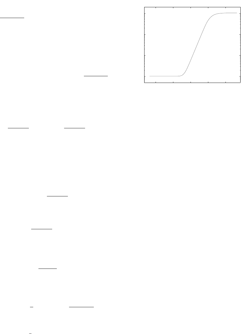
Consequently, the slope of S

as a function of ε on a

log-log scale is

. However, this slope is only linear

in a limited subrange of ε since lim

ε→∞

= m

and

lim

ε→0

= m as illustrated in Fig. 1. In this sub-

range, the error terms in Eq. (7) are smaller than they

are in the rest of the ε range. Thus, an adequate ε

should be chosen from this linear subrange.

−4

−2

log(ε)

log(S

)

Figure 1: A plot of S

as a function of ε on a log-log scale.

NCTA 2015 - 7th International Conference on Neural Computation Theory and Applications

156

REFERENCES

Bourgain, J. (1985). On lipschitz embedding of finite metric