Particle Convergence Time in the PSO Model with Inertia Weight
Krzysztof Trojanowski
2,1
and Tomasz Kulpa
1
1
Cardinal Stefan Wyszy
´
nski University, Faculty of Mathematics and Natural Sciences, Warsaw, Poland
2
Institute of Computer Science, Polish Academy of Sciences, Warsaw, Poland
Keywords:
Particle Swarm, Model with Inertia Weight, Particle Convergence.
Abstract:
Particle Swarm Optimization (PSO) is a powerful heuristic optimization method being subject of continuous
interest. Theoretical analysis of its properties concerns primarily the conditions necessary for guaranteeing its
convergent behaviour. Particle behaviour depends on three groups of parameters: values of factors in a velocity
update rule, initial localization and velocity and fitness landscape. The paper presents theoretical analysis of
the particle convergence properties in the model with inertia weight respectively to different values of these
parameters. A new measure for evaluation of a particle convergence time is proposed. For this measure
an upper bound formula is derived and its four main types of characteristics are discussed. The way of the
characteristics transformations respectively to changes of velocity equation parameters is presented as well.
1 INTRODUCTION
Particle swarm optimization (PSO) (Kennedy and
Eberhart, 1995) belongs to a big family of modern
heuristic optimization methods. A number of versions
of PSO has already been proposed sharing the same
paradigm of stochastic, population-based method of
exploration in the given space of solutions in search-
ing for the best one. In our research we selected one
of the earlier versions of PSO proposed in (Shi and
Eberhart, 1998). Like in other methods, the popula-
tion consists of members called here particles which
represent solutions from the given space. Particles are
also equipped with memories which store attractors,
that is, solutions best found so far by the particles. A
working group of particles controlled by the method
is called a swarm. After the initialization of a swarm
the cycle of iterations performs the search process.
The distinctive features of PSO are: (1) application of
particle memory as well as the mechanism of mem-
ory sharing by groups of neighbouring solutions, (2)
the method of finding new solutions based on the idea
of displacement originated from the real-world. Un-
like other metaheuristics, every iteration consists of
two main steps: particles memory update and the dis-
placement of particles within the space of solutions.
In PSO less-fit particles do not die, that is, there is no
”survival of the fittest” mechanism typical for the evo-
lutionary approach. The rules of displacement make
use of the information from the memory and are ex-
pressed by equations which may differ to each other
for different versions of PSO. Particularly, in the ver-
sion of PSO which we selected for analysis the rules
of displacement use the inertia weight parameter.
Numerous applications of PSO confirmed its use-
fulness and potential but also motivate for study-
ing their theoretical properties. Particularly, a par-
ticle stability analysis is a subject of great inter-
est. One of the main aims is estimation of par-
ticle parameter ranges guaranteing the convergent
movement within the given boundaries of the search
space. For the purpose of theoretical analysis some
assumptions concerning randomness have always to
be made. The most restricted deterministic approach
simply eliminates stochastic coefficients from the ve-
locity equation (Clerc and Kennedy, 2002). Other ap-
proaches implement expected values of the particle
locations (Trelea, 2003; van den Bergh and Engel-
brecht, 2006) (which is called a first order stability
analysis), or the variance of the locations (a second or-
der stability analysis) (Poli, 2009; Liu, 2015; Bonyadi
and Michalewicz, 2015).
In the presented research we study behaviour of a
particle which parameters belong to the ranges guar-
anteing the convergent movement, particularly, we
evaluate the time necessary for a particle to enter the
convergent state. This kind of a swarm property was
already investigated for swarms consisting of a num-
ber of particles (Cleghorn and Engelbrecht, 2014b).
In a series of experiments for different particle config-
urations authors evaluated number of iterations nec-
122
Trojanowski, K. and Kulpa, T..
Particle Convergence Time in the PSO Model with Inertia Weight.
In Proceedings of the 7th International Joint Conference on Computational Intelligence (IJCCI 2015) - Volume 1: ECTA, pages 122-130
ISBN: 978-989-758-157-1
Copyright
c
 2015 by SCITEPRESS – Science and Technology Publications, Lda. All rights reserved

essary to satisfy the assumed convergence condition.
However, in our paper we propose a new method of
evaluation of a particle convergence time based on
the first order stability model of PSO with inertia
weight (van den Bergh and Engelbrecht, 2006) and a
new convergence condition. This means that the anal-
ysis concerns a particle model based on the following
assumptions:
1. the particle moves in one-dimensional search
space — there is no need to consider n-
dimensional velocity vectors due to the fact, that
all the velocity parameters are evaluated individ-
ually for each of the search space coordinates and
they do not influence to each other in any way,
2. random values in the velocity equation are re-
placed by their expected values (e.g., for r ∼
U(0,1) it is 0.5), thus the rules of the particle
movement become deterministic,
3. both the local and the global attractor remain in
the same place of the search space over the entire
time of the modelled particle behaviour,
4. there is just one particle to observe — due to the
previous assumption that global attractor remains
unchanged, no communication between particles
exists in fact,
5. values of parameters in the velocity equation be-
long to the ranges guaranteeing convergent move-
ment of the modelled particle.
Thus stability is defined as:
lim
t→∞
x(t) = y (1)
where y is a constant point in the search space.
The selected model based on the five assumptions
allows to generate convergent trajectories of a parti-
cle over space. However, it has to be stressed that
the shape of the trajectory does not influence the pro-
posed measure and the only important information is
the number of steps necessary for the particle to get
and stay in the sufficiently close neighborhood of y.
The paper consists of five sections. In Section 2
the model of PSO with inertia weight is briefly de-
scribed. Section 3 presents the proposed new measure
of particle convergence time. Discussion of the new
measure properties can be found in Section 4. Sec-
tion 5 concludes the paper.
2 THE PSO MODEL
The PSO model with inertia weight implements the
following velocity and position equations:

v
t+1
= w ·v
t
+ ϕ
1
(y
t
−x
t
) + ϕ
2
(y
∗
t
−x
t
),
x
t+1
= x
t
+ v
t+1
(2)
where ϕ
1
= r
1
c
1
, ϕ
2
= r
2
c
2
, and c
1
,c
2
represent ac-
celeration coefficients, r
1
,r
2
∼U(0,1). In the further
analysis the stochastic components ϕ
1
and ϕ
2
are sub-
stituted by their expected values being equal c
1
/2 and
c
2
/2 respectively. We also assume that both attractors
are constant over time.
From this pair of equations a recursive formula
can be derived (van den Bergh and Engelbrecht,
2006):
x
t+1
= (1 +w−ϕ
1
−ϕ
2
)x
t
−wx
t−1
+ϕ
1
y+ϕ
2
y
∗
(3)
which allows to evaluate the particle location, assum-
ing that its two previous locations and its attractor are
known. This way a basic simplified dynamic system
can be defined:
P
t+1
= M ×P
t
, (4)
where:
• P
t
— the particle state made up of its current po-
sition x
t
and the previous one x
t−1
.
• M — the dynamic matrix whose properties deter-
mine the transformations of the particle state.
Results from dynamic system theory say that the
transformations of the particle state depend on the
eigenvalues of M. Further analysis of the dynamic
matrix originated from Eq. (3) allowed to define the
region in the parameters space were eigenvalues of M
are smaller than 1. All the configuration parameters
sets originated from this region guarantee that the par-
ticles do not diverge during the process of search.
In (van den Bergh and Engelbrecht, 2006) authors
show that the particle equilibrium point is a weighted
average of its personal best y and global best y
∗
posi-
tions:
ϕ
1
y+ϕ
2
y
∗
ϕ
1
+ϕ
2
. However, just for simplicity of calcu-
lations and without loss of generality we can assume,
that y
∗
= y. In this case we can substitute φ for ϕ
1
+ϕ
2
and Eq. (3) is reformulated as follows:
x
t+1
= (1 + w −φ)x
t
−wx
t−1
+ φy (5)
Eventually, the following stable region, that is, a set of
convergent configurations satisfies the following sys-
tem of inequalities was derived:



w > 0 ∧w < 1,
φ > 0,
w > 0.5φ −1
(6)
Since the first presentation of the above-
mentioned boundaries of the stable region a num-
ber of publications appeared discussing the problem
Particle Convergence Time in the PSO Model with Inertia Weight
123

of boundaries definition based on different assump-
tions concerning stochastic components in the veloc-
ity equations and stability of attractors. For more de-
tails the reader is referred to (Kadirkamanathan et al.,
2006; Poli, 2009; Gazi, 2012; Cleghorn and Engel-
brecht, 2014a; Liu, 2015). Particularly, in (Cleghorn
and Engelbrecht, 2014a) a set of inequalities coincid-
ing with Ineq. (6) has been derived. In our research
presented in the further text we implement the sta-
ble region as it is defined by Ineq. (6) having in mind
that constraint w > 0 represents just the intuitive as-
sumption that inertia of a moving object should not be
negative.
3 THE PROPOSED MEASURE
3.1 Particle Convergence Time
Even if the stable region is given, it is also interesting
to know the number of steps necessary for the particle
to obtain its stable state for different configurations
(φ,w). In this case ”obtaining stable state” means that
the distance between current and the next location of
the particle is never greater than the given threshold
value δ.
Lets define a set of natural numbers S(δ) for a
given δ > 0 such that:
s ∈ S(δ) ⇐⇒ |x
t+1
−x
t
| < δ for all t ≥ s. (7)
We define the particle convergence time (pct) for
given δ > 0 as follows:
pct(δ) = min{s ∈S(δ)}. (8)
The particle convergence time pct is the minimal
number of steps necessary for the particle to obtain
its stable state as defined above. For estimation of the
particle convergence time we use Eq. (3).
3.2 Upper Bound Formula for pct
Recurrent equations are difficult to analyse, how-
ever, an explicit closed form of the recurrence rela-
tion Eq. (5) is also known (van den Bergh and Engel-
brecht, 2006):
x
t
= k
1
+ k
2
λ
t
1
+ k
3
λ
t
2
, (9)
where
k
1
= y, (10)
k
2
=
λ
2
(x
0
−x
1
) −x
1
+ x
2
γ(λ
1
−1)
, (11)
k
3
=
λ
1
(x
1
−x
0
) + x
1
−x
2
γ(λ
2
−1)
, (12)
x
2
= (1 + w −φ)x
1
−wx
0
+ φy, (13)
λ
1
=
1 + w −φ + γ
2
, (14)
λ
2
=
1 + w −φ −γ
2
, (15)
γ =
q
(1 + w −φ)
2
−4w. (16)
Thus, the distance between two subsequent values
of the particle locations x
t+1
and x
t
equals:
|x
t+1
−x
t
| = |k
2
λ
t
1
(λ
1
−1) + k
3
λ
t
2
(λ
2
−1)|. (17)
From the triangle inequality it follows that:
|x
t+1
−x
t
|≤|k
2
||λ
1
|
t
|λ
1
−1|+|k
3
||λ
2
|
t
|λ
2
−1|. (18)
We are interested in the minimal number of steps
s after which the condition
|x
t+1
−x
t
| < δ (19)
is satisfied for all t ≥ s. To obtain this we employ the
fact, that:
|a| < δ/2 ∧|b|< δ/2 ⇒|a + b| < δ (20)
where |·| is the absolute value.
Thus, we look for such t
1
and t
2
, that:
|k
2
||λ
1
|
t
1
|(λ
1
−1)| < δ/2, (21)
|k
3
||λ
2
|
t
2
|(λ
2
−1)| < δ/2. (22)
and we get:
t
1
>
lnδ −ln(2|k
2
||λ
1
−1|)
ln|λ
1
|
, (23)
t
2
>
lnδ −ln(2|k
3
||λ
2
−1|)
ln|λ
2
|
. (24)
Now, we define s = max(t
1
,t
2
), where t
1
and t
2
are
minimal natural number satisfying Ineq. (23) and (24)
respectively. From (20), (21) and (22) it follows that
for all t ≥ s the condition (19) is satisfied.
In the case where γ is a complex number consist-
ing of just an imaginary value, that is, when (1 +
w −φ)
2
< 4w, the reasoning presented above may
be simplified. In this case the following is satisfied:
|λ
1
| = |λ
2
| and |λ
1
− 1| = |λ
2
− 1|. Let’s denote:
|λ| = |λ
1
| = |λ
2
| and |λ − 1| = |λ
1
−1| = |λ
2
−1|.
Then, Ineq. (18) can be expressed as:
|x
t+1
−x
t
| ≤ |λ|
t
|λ −1|(|k
2
|+ |k
3
|). (25)
In this case we look for such t that:
|λ|
t
|λ −1|(|k
2
|+ |k
3
|) < δ, (26)
which is equivalent to
t >
lnδ −ln(|λ −1|(|k
2
|+ |k
3
|))
ln|λ|
, (27)
ECTA 2015 - 7th International Conference on Evolutionary Computation Theory and Applications
124

Now, we define s as a minimal natural number t
satisfying Ineq. (27). From (25) an (27) it follows that
for all t ≥ s the condition (19) is satisfied.
For both cases, that is, real and imaginary value of
γ, the defined number of steps s satisfies condition (7).
Due to the fact, that pcs(δ) is defined as a minimal
number satisfying condition (7), we get pcs(δ) ≤ s.
Thus, Ineq. (23), (24) and (27) give us the ana-
lytic upper bounds for the particle convergence time,
which is denoted as pctb(δ). The explicit formula for
pctb(δ) is
pctb(δ) = max

lnδ −ln(2|k
2
||λ
1
−1|)
ln|λ
1
|
,
lnδ −ln(2|k
3
||λ
2
−1|)
ln|λ
2
|

(28)
for real value of γ and
pctb(δ) =
lnδ −ln(|λ −1|(|k
2
|+ |k
3
|))
ln|λ|
(29)
for imaginary value of γ.
4 VISUALIZATIONS OF PCT B
CHARACTERISTICS
Particle convergence time depends on three groups of
parameters: values of factors in a velocity update rule,
initial localization and velocity and fitness landscape.
Parameters from the first group, that is, φ and w define
character (or temperament) of a particle. An exam-
ple graph of pctb(φ, w) is presented in the subsection
below. The next subsection presents example graphs
of pctb(x
0
,x
1
), that is, convergence times of particles
with selected characters respectively to their starting
conditions. Particle trajectories for respective types
of character are also presented. The third subsection
shows how pctb(x
0
,x
1
) and pctb(x
0
,v) graphs vary
respectively to the changes in a particle character.
4.1 Particle Convergence Time for
Different Types of Particles
The characteristics of pctb as a function of parti-
cle configuration parameters φ and w share common
shape presented in Figure 1. The Figure depicts the
pctb(φ,w) characteristic obtained from a grid of eval-
uation points starting from a configuration [φ = 0.025,
w = 0.044] and changing with step 0.05 in both di-
rections. This choice of method for the function
graph generation is due to the fact, that γ appears
in the denominator of Eq. (11) and (12), so, it can-
not equal zero. Unfortunately, this is the case, when
w = 1 + φ −2
√
φ, that is, there exist points in the sta-
ble region for which the upper bound for their conver-
gence time can be evaluate neither with formula (28)
nor (29).
For better visibility the pctb(φ,w) axis has loga-
rithmic scale and the evaluation points from outside
the stable region have assigned the constant value
5000.
0
1
2
3
4
0
0.5
1
1
10
100
1000
φ
w
0
500
1000
1500
2000
2500
3000
3500
4000
4500
5000
5500
Figure 1: Particle convergences pctb(φ,w) for example
starting conditions: x
0
= 1 and x
1
= −8.1.
Figure 1 shows that when the inertia weight w
is low the convergence times are also low and in-
crease as the inertia grows. Additionally, pctb in-
creases also for the cases when acceleration coeffi-
cient φ approaches boundary values, both left and
right, however, for the right boundary the increase is
much higher than for the left.
4.2 pctb as a Function of Initial
Location and Velocity
For φ and w values satisfying Ineq. (6) the shapes of
pctb(x
0
,x
1
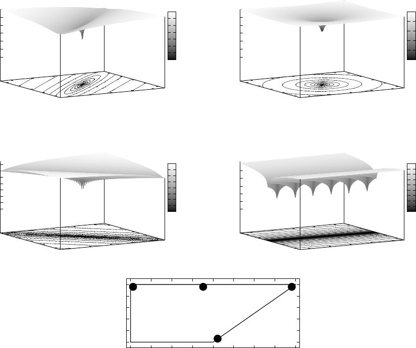
) can be classified into four main types.
Their representatives for δ = 0.0001 are depicted in
Figure 2:
A: convergence is fast when the velocity is low (x
1
close to x
0
) and the initial location x
0
is irrelevant
in every case;
B: a transitional state between states A and C;
C: convergence is fast when the velocity is adjusted
to the location and directed toward the attractor;
D: the particle has almost no inertia, so, the less dis-
tance from x
1
to the attractor, the less value of
pctb.
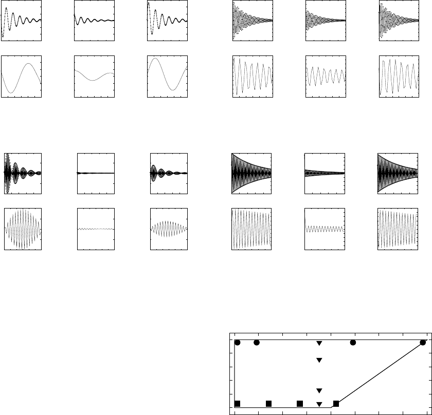
Figure 3 shows subsequent locations of particles
over time for particle configurations selected for pre-
sentation in Figure 2 and for three different starting
locations each. Graphs of particle trajectories similar
to the ones presented in Figure 3 can be also found
in (Trelea, 2003), however, in that case they were ob-
tained for different particle parameter space. Graphs
Particle Convergence Time in the PSO Model with Inertia Weight
125

-8
-4
0
4
8
-8
-4
0
4
8
0
100
200
300
400
500
600
w=0.96; φ=0.06; y=0
x
0
x
1
250
300
350
400
450
500
550
600
(a) type A
-8
-4
0
4
8
-8
-4
0
4
8
0
100
200
300
400
500
600
w=0.96; φ=1.76; y=0
x
0
x
1
350
400
450
500
550
600
(b) type B
-8
-4
0
4
8
-8
-4
0
4
8
0
100
200
300
400
500
600
700
w=0.96; φ=3.91; y=0
x
0
x
1
350
400
450
500
550
600
650
700
750
(c) type C
-8
-4
0
4
8
-8
-4
0
4
8
0
200
400
600
800
1000
1200
w=0.06; φ=2.11; y=0
x
0
x
1
400
500
600
700
800
900
1000
1100
1200
1300
(d) type D
0
0.2
0.4
0.6
0.8
1
0 0.5 1 1.5 2 2.5 3 3.5 4
A B
C
D
(e) localizations of selected configurations for types A,
B, C and D in the configuration space (φ,w)
Figure 2: Graphs of pctb(x
0
,x
1
) for selected configurations (φ,w) which represent four types of characteristics: A, B, C and
D.
with trajectories can be also found in other publica-
tions, particularly in (van den Bergh and Engelbrecht,
2006), however, they are not classified respectively to
the subarea in the stable region of the configuration
space they appear.
In Figure a ”A” particles are represented by three
cases: with low (starting points x
0
and x
1
at (8,8.1))
and high initial velocity: ((8,1.1) and (1,8.1)). High
inertia and weak attraction toward y make the move-
ment smooth and the subsequent steps short in every
case. For the high initial velocity oscillations around
the attractor are higher. In the case of ”B” particles
(Figure b) oscillations appear in every graph, how-
ever, the length of subsequent steps is irregular: when
the particle moves away from y with high velocity,
sometimes the attracting force almost stops it, ve-
locity decreases and the particle turns back slowly,
whereupon runs toward the attractor with a high ve-
locity again. Figure c presents a ”zig-zag” trajectories
of ”C” particles which amplitude cyclically increases
and decreases. The amplitude of oscillations is less
when the initial velocity is adjusted to the initial lo-
cation and directed toward the attractor. Clearly, the
fastest convergence of pctb is obtained when x
1
has
the same absolute value as x
0
but the opposite sign.
Figure d also presents a ”zig-zag” trajectories of ”D”
particles but without cycles in the magnitude of am-
plitude. In this case particle also converges to the at-
tractor faster when the initial velocity is adjusted to
the initial location, however, in this case the veloc-
ECTA 2015 - 7th International Conference on Evolutionary Computation Theory and Applications
126

-30
-20
-10
0
10
20
30
0 30 60 90 120 150
x(t)
x
0
=8.0; x
1
=1.1;
-30
-20
-10
0
10
20
30
0 30 60 90 120 150
x(t)
x
0
=8.0; x
1
=8.1;
-30
-20
-10
0
10
20
30
0 30 60 90 120 150
x(t)
x
0
=1.0; x
1
=8.1;
-30
-20
-10
0
10
20
30
0 5 10 15 20 25 30
x(t)
t
-30
-20
-10
0
10
20
30
0 5 10 15 20 25 30
x(t)
t
-30
-20
-10
0
10
20
30
0 5 10 15 20 25 30
x(t)
t
(a) type A: (x
0
,x
1
) ∈{(8,1.1), (8, 8.1),(1,8.1)}
-10
-8
-6
-4
-2
0
2
4
6
8
10
0 30 60 90 120 150
x(t)
x
0
=4.0; x
1
=9.0;
-10
-8
-6
-4
-2
0
2
4
6
8
10
0 30 60 90 120 150
x(t)
x
0
=4.0; x
1
=4.0;
-10
-8
-6
-4
-2
0
2
4
6
8
10
0 30 60 90 120 150
x(t)
x
0
=4.0; x
1
=-9.0;
-10
-8
-6
-4
-2
0
2
4
6
8
10
0 5 10 15 20 25 30
x(t)
t
-10
-8
-6
-4
-2
0
2
4
6
8
10
0 5 10 15 20 25 30
x(t)
t
-10
-8
-6
-4
-2
0
2
4
6
8
10
0 5 10 15 20 25 30
x(t)
t
(b) type B: (x
0
,x
1
) ∈{(4,9), (4, 4),(4,−9)}
-100
-50
0
50
100
0 30 60 90 120 150
x(t)
x
0
=4.0; x
1
=9.0;
-100
-50
0
50
100
0 30 60 90 120 150
x(t)
x
0
=4.0; x
1
=-4.0;
-100
-50
0
50
100
0 30 60 90 120 150
x(t)
x
0
=4.0; x
1
=-9.0;
-100
-50
0
50
100
0 5 10 15 20 25 30
x(t)
t
-100
-50
0
50
100
0 5 10 15 20 25 30
x(t)
t
-100
-50
0
50
100
0 5 10 15 20 25 30
x(t)
t
(c) type C: (x
0
,x
1
) ∈{(4,9), (4, −4),(4,−9)}
-10
-8
-6
-4
-2
0
2
4
6
8
10
0 30 60 90 120 150
x(t)
x
0
=4.0; x
1
=9.0;
-10
-8
-6
-4
-2
0
2
4
6
8
10
0 30 60 90 120 150
x(t)
x
0
=9.0; x
1
=1.0;
-10
-8
-6
-4
-2
0
2
4
6
8
10
0 30 60 90 120 150
x(t)
x
0
=4.0; x
1
=-9.0;
-10
-8
-6
-4
-2
0
2
4
6
8
10
0 5 10 15 20 25 30
x(t)
t
-10
-8
-6
-4
-2
0
2
4
6
8
10
0 5 10 15 20 25 30
x(t)
t
-10
-8
-6
-4
-2
0
2
4
6
8
10
0 5 10 15 20 25 30
x(t)
t
(d) type D: (x
0
,x
1
) ∈{(4,9), (9, 1),(4,−9)}
Figure 3: Particle trajectories for the four types of characteristics: A, B, C and D, and for three example starting locations;
a view of 150 locations (top figures) and a close-up of the first 30 locations (bottom figures).
ity has to be adjusted so as to locate x
1
in the near-
est neighborhood of the attractor. Finally, it is worth
noting that different types of trajectories appear for
different types of particle characteristics, which con-
firms the proposed selection of types and allows one
to assume that none of the selected types is a subtype
of any other.
4.3 Transformations of pctb
Characteristics
The four types of characteristics transform smoothly
from one to another when the φ and w parameters
vary. Example series Q1, Q2 and Q3 of pctb graph
pairs: pctb(x
0
,x
1
) and pctb(x
0
,v) for δ = 0.0001 are
presented in Figures 5, 6 and 7 respectively. Local-
izations of selected series of configurations: Q1, Q2
and Q3 in the configuration space (φ,w) are depicted
in Figure 4.
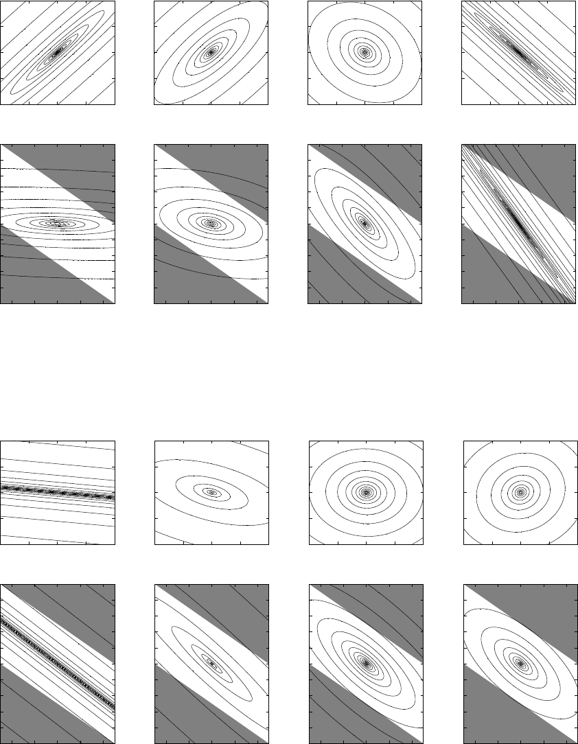
In Figure 5 the first series of figures called Q1
shows the transformations when the inertia weight
w is high, that is, w = 0.96 and φ varies from min-
imal to maximal values within the stability region:
φ ∈ {0.06,0.46,2.46,3.91}. For small values of φ the
most important for pctb is the initial velocity: when
0
0.2
0.4
0.6
0.8
1
0 0.5 1 1.5 2 2.5 3 3.5 4
Q11 Q12 Q13 Q14
Q21
Q22
Q23
Q24
Q31 Q32 Q33 Q34
Figure 4: Localizations of configuration series presented in
top three rows of pictures: Q1 (marked as circles), Q2 (tri-
angles), and Q3 (squares) in the configuration space (φ,w).
it is small, the pctb is low, otherwise, the number of
steps necessary to reach the attractor grows rapidly.
On the opposite end of series Q1 one can observe the
case when for small values of pctb the velocity should
be adjusted to the distance to the attractor. The further
is the particle from the attractor, the higher initial ve-
locity is needed to reach the attractor in small number
of steps. In every case the velocity must be directed
toward the attractor.
In Figure 6 the series Q2 is presented. The at-
tractor coefficient is fixed, that is, φ = 1.76 and the
inertia weight varies: w ∈ {0.06,0.26,0.71, 0.96}. In
every case for the sake of pctb minimization the ini-
Particle Convergence Time in the PSO Model with Inertia Weight
127

w=0.96; φ=0.06; y=0; pctb: [0,600]
-0.1 -0.05 0 0.05 0.1
x
0
-0.1
-0.05
0
0.05
0.1
x
1
w=0.96; φ=0.06; y=0; pctb: [0,600]
-8 -4 0 4 8
x
0
-20
-16
-12
-8
-4
0
4
8
12
16
20
v
(a) Q11
w=0.96; φ=0.46; y=0; pctb: [0,600]
-0.1 -0.05 0 0.05 0.1
x
0
-0.1
-0.05
0
0.05
0.1
x
1
w=0.96; φ=0.46; y=0; pctb: [0,600]
-8 -4 0 4 8
x
0
-20
-16
-12
-8
-4
0
4
8
12
16
20
v
(b) Q12
w=0.96; φ=2.46; y=0; pctb: [0,650]
-0.1 -0.05 0 0.05 0.1
x
0
-0.1
-0.05
0
0.05
0.1
x
1
w=0.96; φ=2.46; y=0; pctb: [0,650]
-8 -4 0 4 8
x
0
-20
-16
-12
-8
-4
0
4
8
12
16
20
v
(c) Q13
w=0.96; φ=3.91; y=0; pctb: [0,750]
-0.1 -0.05 0 0.05 0.1
x
0
-0.1
-0.05
0
0.05
0.1
x
1
w=0.96; φ=3.91; y=0; pctb: [0,750]
-8 -4 0 4 8
x
0
-20
-16
-12
-8
-4
0
4
8
12
16
20
v
(d) Q14
Figure 5: Particle convergence times pctb for a series Q1: fixed w = 0.96 and φ ∈ {0.06,0.46,2.46, 3.91}; the top fig-
ures: pctb(x
0
,x
1
); the bottom figures: pctb(x
0
,v); the white area in figures for pctb(x
0
,v) maps to the domain defined for
pctb(x
0
,x
1
).
w=0.06; φ=1.76; y=0; pctb: [0,30]
-0.1 -0.05 0 0.05 0.1
x
0
-0.1
-0.05
0
0.05
0.1
x
1
w=0.06; φ=1.76; y=0; pctb: [0,30]
-8 -4 0 4 8
x
0
-20
-16
-12
-8
-4
0
4
8
12
16
20
v
(a) Q21
w=0.26; φ=1.76; y=0; pctb: [0,30]
-0.1 -0.05 0 0.05 0.1
x
0
-0.1
-0.05
0
0.05
0.1
x
1
w=0.26; φ=1.76; y=0; pctb: [0,30]
-8 -4 0 4 8
x
0
-20
-16
-12
-8
-4
0
4
8
12
16
20
v
(b) Q22
w=0.71; φ=1.76; y=0; pctb: [0,75]
-0.1 -0.05 0 0.05 0.1
x
0
-0.1
-0.05
0
0.05
0.1
x
1
w=0.71; φ=1.76; y=0; pctb: [0,75]
-8 -4 0 4 8
x
0
-20
-16
-12
-8
-4
0
4
8
12
16
20
v
(c) Q23
w=0.96; φ=1.76; y=0; pctb: [0,600]
-0.1 -0.05 0 0.05 0.1
x
0
-0.1
-0.05
0
0.05
0.1
x
1
w=0.96; φ=1.76; y=0; pctb: [0,600]
-8 -4 0 4 8
x
0
-20
-16
-12
-8
-4
0
4
8
12
16
20
v
(d) Q24
Figure 6: Particle convergence times pctb for a series Q2: fixed φ = 1.76 and w ∈ {0.06,0.26,0.71, 0.96}; the top fig-
ures: pctb(x
0
,x
1
); the bottom figures: pctb(x
0
,v); the white area in figures for pctb(x
0
,v) maps to the domain defined for
pctb(x
0
,x
1
).
ECTA 2015 - 7th International Conference on Evolutionary Computation Theory and Applications
128

w=0.06; φ=0.06; y=0; pctb: [0,150]
-0.1 -0.05 0 0.05 0.1
x
0
-0.1
-0.05
0
0.05
0.1
x
1
w=0.06; φ=0.06; y=0; pctb: [0,150]
-8 -4 0 4 8
x
0
-20
-16
-12
-8
-4
0
4
8
12
16
20
v
(a) Q31
w=0.06; φ=0.71; y=0; pctb: [0,10]
-0.1 -0.05 0 0.05 0.1
x
0
-0.1
-0.05
0
0.05
0.1
x
1
w=0.06; φ=0.71; y=0; pctb: [0,10]
-8 -4 0 4 8
x
0
-20
-16
-12
-8
-4
0
4
8
12
16
20
v
(b) Q32
w=0.06; φ=1.36; y=0; pctb: [0,10]
-0.1 -0.05 0 0.05 0.1
x
0
-0.1
-0.05
0
0.05
0.1
x
1
w=0.06; φ=1.36; y=0; pctb: [0,10]
-8 -4 0 4 8
x
0
-20
-16
-12
-8
-4
0
4
8
12
16
20
v
(c) Q33
w=0.06; φ=2.11; y=0; pctb: [0,1250]
-0.1 -0.05 0 0.05 0.1
x
0
-0.1
-0.05
0
0.05
0.1
x
1
w=0.06; φ=2.11; y=0; pctb: [0,1250]
-8 -4 0 4 8
x
0
-20
-16
-12
-8
-4
0
4
8
12
16
20
v
(d) Q34
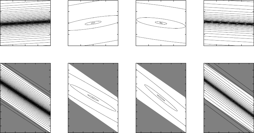
Figure 7: Particle convergence times pctb for a series Q3: fixed w = 0.06 and φ ∈ {0.06,0.71,1.36, 2.11}; the top fig-
ures: pctb(x
0
,x
1
); the bottom figures: pctb(x
0
,v); the white area in figures for pctb(x
0
,v) maps to the domain defined for
pctb(x
0
,x
1
).
tial velocity should be adjusted to the initial location
of the particle. However, for small values of the in-
ertia weight a small error in adjustment causes large
increase of pctb value, whereas, large values of iner-
tia make this change less abrupt, that is, the system is
more stable.
The series of characteristics Q3 is depicted in Fig-
ure 7. In this case the inertia weight w is low, that is,
w = 0.06 and φ ∈ {0.06,0.71, 1.36,2.11}. As it is in
the series Q1, when φ is small the initial location is
almost negligible and the most influential parameter
is velocity: when v is close to zero, the pctb is the
smallest. In the Q3 series the boundary cases repre-
sent configurations sensitive to the error of velocity
vs. location adjustment, that is, the stability of these
configurations is low. The most stable configurations
are the ones in the middle of the range.
Finally, note, that the three series have two shared
configurations. Q21 may belong also to Q3: this con-
figuration can be located between Q33 and Q34. Q24
may belong to Q1 and located between Q12 and Q13.
When we take a look at all the series, one can also
observe that in most cases the pctb is sensitive to an
error in the adjustment particularly for the largest val-
ues of φ both for small and high values of w (partic-
ularly, the examples Q14, Q21, and Q34). The most
stable configurations, that is, resistant to lack of ap-
propriate adjustment of parameters can be found in
the middle of the series Q2, particularly Q24. It is
worth noting here, that one of the popular choices
of particle parameters: c
1
= c
2
= 1.49445 and w =
0.72984 (in (Eberhart and Shi, 2000) authors showed
that the two values lead to satisfying results for a se-
ries of benchmark functions) belongs to the area of
such a stable configurations. On the other side, for
the smallest values of φ the initial location of a parti-
cle has no significant influence and pctb depends on
just the velocity: the smaller v the less pctb.
5 CONCLUSIONS
In the presented research for a model of PSO with
inertia weight we propose a new measure of particle
convergence time (pct). The measure evaluates num-
ber of steps necessary for a particle to obtain a stable
state defined with any precision. For this measure an
upper bound formula (pctb) is derived and its prop-
erties are studied. Particularly, for the particle con-
figurations from the convergence region of the (φ,w)
space four main types of characteristics are identified.
Additionally, we show the way of transformation be-
tween the characteristic shapes when the parameters
φ and w vary.
Particle Convergence Time in the PSO Model with Inertia Weight
129

In the future work we can use the obtained results,
for example, for development of heterogenous parti-
cle swarm optimizers. The idea of swarms where par-
ticles may vary its behaviour during the process of
search can be found in the literature (see, e.g, (Engel-
brecht, 2010; Li and Yang, 2010; Nepomuceno and
Engelbrecht, 2013a; Nepomuceno and Engelbrecht,
2013b)). Now, using the measure presented in this
paper it can be easier to identify requested particle
properties and develop strategies of particle configu-
ration adaptation respectively to the search progress
and current state of particles in a swarm.
REFERENCES
Bonyadi, M. R. and Michalewicz, Z. (2015). Analysis of
stability, local convergence, and transformation sensi-
tivity of a variant of particle swarm optimization algo-
rithm. IEEE T. Evolut. Comput. Date of Publication:
July 25, 2015.
Cleghorn, C. W. and Engelbrecht, A. P. (2014a). A gener-
alized theoretical deterministic particle swarm model.
Swarm Intelligence, 8(1):35–59.
Cleghorn, C. W. and Engelbrecht, A. P. (2014b). Par-
ticle swarm convergence: An empirical investiga-
tion. In Evolutionary Computation (CEC), 2014 IEEE
Congress on, pages 2524 – 2530. IEEE Press.
Clerc, M. and Kennedy, J. (2002). The particle swarm-
explosion, stability, and convergence in a multidi-
mensional complex space. IEEE T. Evolut. Comput.,
6(1):58–73.
Eberhart, R. C. and Shi, Y. (2000). Comparing inertia
weights and constriction factors in particle swarm op-
timization. In Proc. of the 2000 Congress on Evo-
lutionary Computation, pages 84–88, Piscataway, NJ.
IEEE Service Center.
Engelbrecht, A. P. (2010). Heterogeneous particle swarm
optimization. In Swarm Intelligence, volume 6234 of
Lecture Notes in Computer Science, pages 191–202.
Springer Berlin Heidelberg.
Gazi, V. (2012). Stochastic stability analysis of the particle
dynamics in the pso algorithm. In Intelligent Control
(ISIC), 2012 IEEE International Symposium on, pages
708 – 713. IEEE Press.
Kadirkamanathan, V., Selvarajah, K., and Fleming, P. J.
(2006). Stability analysis of the particle dynamics in
particle swarm optimizer. IEEE T. Evolut. Comput.,
10(3):245–255.
Kennedy, J. and Eberhart, R. C. (1995). Particle swarm op-
timization. In Proc. of the IEEE Int. Conf. on Neural
Networks, pages 1942–1948, Piscataway, NJ. IEEE.
Li, C. and Yang, S. (2010). Adaptive learning particle
swarm optimizer-II for global optimization. In IEEE
Congress on Evolutionary Computation, pages 1–8.
IEEE.
Liu, Q. (2015). Order-2 stability analysis of particle swarm
optimization. Evol. Comput., 23(2):187–216.
Nepomuceno, F. V. and Engelbrecht, A. P. (2013a). Be-
havior changing schedules for heterogeneous parti-
cle swarms. In Computational Intelligence and 11th
Brazilian Congress on Computational Intelligence,
2013 BRICS Congress on, pages 112 – 118. IEEE
Press.
Nepomuceno, F. V. and Engelbrecht, A. P. (2013b). A self-
adaptive heterogeneous PSO for real-parameter opti-
mization. In 2013 IEEE Conference on Evolutionary
Computation, volume 1, pages 361–368.
Poli, R. (2009). Mean and variance of the sampling distri-
bution of particle swarm optimizers during stagnation.
IEEE T. Evolut. Comput., 13(4):712–721.
Shi, Y. and Eberhart, R. C. (1998). A modified parti-
cle swarm optimizer. In Proceedings of the IEEE
Congress on Evolutionary Computation 1998, pages
69–73. IEEE Press.
Trelea, I. C. (2003). The particle swarm optimization algo-
rithm: convergence analysis and parameter selection.
Inform. Process. Lett., 85(6):317 – 325.
van den Bergh, F. and Engelbrecht, A. P. (2006). A study of
particle swarm optimization particle trajectories. In-
form. Sciences, 176(8):937–971.
ECTA 2015 - 7th International Conference on Evolutionary Computation Theory and Applications
130