Word Sense Discrimination on Tweets: A Graph-based Approach
Flavio Massimiliano Cecchini, Elisabetta Fersini and Enza Messina
DISCo, University of Milano-Bicocca, Viale Sarca 336, 20126, Milan, Italy
Keywords:
Word Sense Discrimination, Graphs, Twitter.
Abstract:
In this paper we are going to detail an unsupervised, graph-based approach for word sense discrimination on
tweets. We deal with this problem by constructing a word graph of co-occurrences. By defining a distance
on this graph, we obtain a word metric space, on which we can apply an aggregative algorithm for word
clustering. As a result, we will get word clusters representing contexts that discriminate the possible senses of
a term. We present some experimental results both on a data set consisting of tweets we collected and on the
data set of task 14 at SemEval-2010.
1 INTRODUCTION
In the wide research field of Natural Language Pro-
cessing, the task of Word Sense Disambiguation
(WSD) is that of unravelling the intrinsic arbitrari-
ness of human language to provide a better under-
standing of text or speech. In particular, the case of
proper nouns can be very challenging, since the cor-
relation between a name and the object, person, loca-
tion or the like it denotes is often more obscure and
unpredictable than e.g. the continuous shift in mean-
ing of common nouns. This task is even more com-
plex when dealing with text on social networks (e.g.
tweets), where shortness and informal writing styles
represent an additional challenge. Many approaches
in Word Sense Disambiguation are supervised, that is,
they resolve to use some kind of external knowledge
about the world to discern the possible senses that a
given term can assume in the discourse. Concerning
the state of the art, several approaches have been pro-
posed for well-formed, i.e. grammatically and ortho-
graphically correct text. Three main research direc-
tions have been investigated (Navigli, 2009), (Navigli,
2012): 1) supervised (Zhong and Ng, 2010), (Mihal-
cea and Faruque, 2004), 2) knowledge-based (Nav-
igli and Ponzetto, 2012), (Schmitz et al., 2012) and
3) unsupervised Word Sense Disambiguation (Dorow
and Widdows, 2003), (V
´
eronis, 2004), (Biemann,
2006), (Hope and Keller, 2013) where the last ap-
proach is better defined as “induction” or “discrim-
ination”. These approaches try to cluster a generic
word graph: in (Biemann, 2006) a simplified variant
of Markov clustering (Chinese Whispers) is used to
reproduce the propagation of a sense from one word
to the others; in (V
´
eronis, 2004), the concept of den-
sity and hub words is used, and the more recent pro-
posal by (Hope and Keller, 2013) permits soft cluster-
ing in linear time. To the best of our knowledge, many
of these works apply a quite selective choice of words
on an underlying corpus when building a graph, and
make thereby more or less implicit assumptions on
the domain or format of the text, like the frequency of
certain syntactical constructions.
In this paper we focus on the automatic discov-
ery of senses from raw text, by pursuing an unsu-
pervised Word Sense Discrimination paradigm. We
are interested in the development of a method that
can be generally independent from the register or
the linguistic well-formedness of a text document,
and, given an adequate pre-processing step, from lan-
guage. Among the many unsupervised research di-
rections, i.e. context clustering (Sch
¨
utze, 1998), word
clustering (Lin, 1998), probabilistic clustering (Brody
and Lapata, 2009) and co-occurrence graph cluster-
ing (Widdows and Dorow, 2002), we committed to
the last one, based on the assumption that word co-
occurrence graphs can reveal local structural proper-
ties tied to the different senses a word might assume
in different contexts.
The structure of the paper is as follows. In Section
2 we present the framework of our approach and ex-
plain all passages and constructions in detail; in Sec-
tion 3 we describe the clustering algorithm; and fi-
nally, in Section 4 we show the results obtained both
on our custom tweet data set and on SemEval-2010,
Task 14’s data set. Section 5 concludes the paper.
138
Cecchini, F., Fersini, E. and Messina, E..
Word Sense Discrimination on Tweets: A Graph-based Approach.
In Proceedings of the 7th International Joint Conference on Knowledge Discovery, Knowledge Engineering and Knowledge Management (IC3K 2015) - Volume 1: KDIR, pages 138-146
ISBN: 978-989-758-158-8
Copyright
c
2015 by SCITEPRESS – Science and Technology Publications, Lda. All rights reserved
2 OVERVIEW AND DEFINITIONS
2.1 Overview
In the approach that we are going to propose for word
sense disambiguation, or better discrimination, we go
through four main steps:
• word filtering of the text documents;
• construction of a co-occurrence word graph;
• derivation of metric word spaces from the graph;
• and finally the clustering algorithm.
Word filtering is a necessary step to remove all the
words that are of no interest to our goal and that would
otherwise just generate noise; it is a fact that only a
few words are truly relevant to the conveyance of the
general sense of a discourse, and word filtering helps
us restrict our attention to those few selected words.
The co-occurence graph (and its subgraphs) will serve
us as a representation of the underlying structure of
the text documents (tweets) we are considering. From
there, it is possible to extract contexts
1
of a word v
we want to disambiguate. By comparing the con-
texts of two words, we can define a graph-based dis-
tance between words and derive a word metric space
from it. Even if it is not possible to visualize this
space as some canonical R
n
, we can still run clus-
tering algorithms on it, like e.g. k-medoids or similar
ones. Our basic assumption is that the word space that
arises from the context of a term v we want to disam-
biguate will present denser areas that we want to iden-
tify through clustering. Each one of these agglom-
erates will then implicitly define a different sense of
term v. Our assumptions imply that, even if the possi-
ble senses that a word can assume are not predictable
a priori and could vary from tweet to tweet
2
, in every
single sentence that word will not display any ambi-
guity; that is, every word can be ambiguous a pri-
ori, but the context it is used together defines its sense
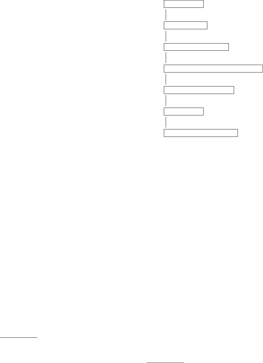
there unequivocally. We show a high-level overview
of our proposed approach in Figure 1.
2.2 Word Filtering
Before building the co-occurrence graph, we want to
filter out functional words that do not carry a mean-
1
The context of a word will mostly consist of all the
words that co-occur with it in the same tweet, sentence, or
whichever textual unit is chosen.
2
Since we are using a data set consisting of tweets, we
consider a tweet the basic textual unit where a word has to
be disambiguated. With other types of documents, we could
instead consider sentences, paragraphs, or what is deemed
as the most adequate choice.
Tweets
Reduced tweets
Word graph of all tweets
Word cloud of term to disambiguate
Word cloud’s metric space
Sense clusters
Disambiguated original text
?
?
?
?
?
?
Cluster labelling
Aggregative clustering algorithm
Weighted Jaccard distance
Neighbourhood’s subgraph
Graph construction
Word filtering
Figure 1: Framework of the proposed disambiguation pro-
cess.
ing by themselves (so-called stop words) or that are
not significant enough to our ends. We therefore
apply a first filtering step based on stop word lists
and part-of-speech tagging. First, we remove easily
identifiable common stop words, mostly closed-class
3
words like articles (the, a, . . . ), prepositions (of, to,
. . . ), conjunctions (and, but, . . . ) and so on, but also
modal verbs (can, will, . . . ). A difficulty encountered
dealing with tweets is the often irregular or idiosyn-
cratic spelling of words, a fact whose consequence is
that many closed word classes graphically assume the
traits of open classes. Therefore, the preposition for
could appear as fir, fr, fo, 4, and be hardly recog-
nizable as such. To overcome this complication, we
used the ARK POS tagger for Twitter (Owoputi et al.,
2013), based on word clusters. Only what is classified
as a noun, a proper noun, a verb or a hashtag (later
the # symbol will be removed) is kept, thus exclud-
ing all closed-class words (prepositions, conjunctions,
articles, . . . ), adverbs and adjectives (since we are not
interested in the “sentiment” of the tweets), mentions
of other users (through the @ symbol), emoticons (in
some sense a graphical equivalent of adverbs), URLs,
numerals, punctuation and other generic noise. We
also want to remove clitics like in Dana’ll, John’s,
and so on.
It has to be remarked that word filtering is a
3
Closed word classes are those whose elements are fixed
and of which no new one is produced by the language, at
least from a synchronic point of view. They are often func-
tion words.
Word Sense Discrimination on Tweets: A Graph-based Approach
139

highly language-dependent step, and its implementa-
tion heavily depends on many ad hoc solutions and
decisions.
Principal Component Analysis
The greatly reduced tweets we obtain this way still
contain many terms that do not carry a useful enough
meaning for our disambiguation task: most of the
context is actually irrelevant. To this end, we further
reduce our vocabulary by means of principal com-
ponent analysis. Given a term we want to disam-
biguate, we want to refine the vocabulary of all the
documents, in our case tweets, where it appears. We
build a TF-IDF matrix where each row represents one
of the selected tweets, each column a word in those
tweets’ vocabulary V
T
, and each entry the TF-IDF
score of the corresponding word w in the tweet, pos-
sibly 0 if it doesn’t appear there. The more the score
of a single word (seen as a random variable) varies
across the tweets, the more we deem it to be rele-
vant for disambiguation. The first principal compo-
nent Y =
∑
w∈V
T
α
w
· w obtained from the covariance
matrix is by definition the linear combination of word
random variables with maximum variance between
all possible linear combinations of word random vari-
ables. We want to retain only the words which con-
tribute the most to the first principal component: that
is, we will retain a word w if and only if |α
w
| > µ,
where µ is the mean of the absolute values of Y’s lin-
ear coefficients.
2.3 The Co-occurrence Graph
Given a collection of tweets, a co-occurrence word
graph can be defined as an undirected, weighted graph
G = (V
G
,E
G
), where the set of vertices V
G
corre-
sponds to the vocabulary of the tweets and two nodes,
i.e. words or tokens, are connected by an edge if and
only if they co-occur in the same tweet. The weight
of that edge is the number of such co-occurrences. It
is interesting to note how all the words in the same
tweet will be connected to each other, so that each
tweet with k different words appearing in the docu-
ments will be represented by a clique of k nodes in
the graph G; this means that G can be considered as
arising from gluing many cliques of different sizes
along their common nodes
4
. Another property of G,
and of word graphs in general (i Cancho and Sol
´
e,
2001), is its small-world (Watts and Strogatz, 1998)
and probably scale-free structure. By “small world”
4
From this point of view, G could be seen as a particu-
lar case of CW-complex construction (Fritsch and Piccinini,
1990).
we mean that the graph has a radically different distri-
bution than what would be expected from a randomly
generated graph on the same set of nodes. The small-
world structure of G reflects syntactical and lexical
rules that underlie the formation of utterances in natu-
ral languages. In particular, a small-world graph is de-
fined as having a very short average shortest path (the
famous “six degrees of separation”), but a high aver-
age clustering coefficient
5
; furthermore, “scale-free”
means that node degrees are distributed according to
a power law, so that there are just a few nodes with
very high degrees that act as “hubs” for the paths in
the graph. In other words, the graph is locally very co-
hesive and globally hinges on few nodes from which
nearly every other node can be reached. This fact can
be interpreted noting that language itself hinges on
some particular words (or better, morphemes) to ex-
press grammatical and syntactical dependencies (e.g.
the, of, that, in English), or tends to recur to words
with a more prototypical or general meaning than oth-
ers (e.g. dog vs. pitbull) (G
¨
ardenfors, 2004).
Word Clouds
The set of nodes V
G
of the graph G encompasses all
the words appearing in our filtered text documents.
However, when disambiguating a term v, we will only
focus on a specific open neighbourhood of v, i.e. its
word cloud, defined as follows:
Definition 1. The word cloud G
v
of v is its n-th de-
gree open neighbourhood graph (or “ego graph”),
consisting of the subgraph of G induced by all the
nodes no more than n steps away from v, excluding
v itself.
The global graph G will serve us as the underly-
ing structure from which we will extract local sub-
graphs that represent the contexts of the words we are
interested in disambiguating. We are not including v
in its neighbourhood, since the resulting word cloud
would be warped around it and resemble a star graph:
v would have the highest degree and be the most cen-
tral node in G
v
. Since we are interested in investigat-
ing the relations between words in the context of v, we
are going to remove v from its neighbourhood as an
interfering factor. In our work, we will just consider
1 as the neighbourhood’s degree, thus taking into ac-
count only nodes adjacent to v.
5
The clustering coefficient for a node v is defined as the
ratio of the number of all existing edges between any two
nodes in the open neighbourhood of v to the maximum pos-
sible number of those edges.
KDIR 2015 - 7th International Conference on Knowledge Discovery and Information Retrieval
140
2.4 The Word Metric Space
Given a generic word graph F = (V
F
,E
F
), in order for
the vocabulary V
F
to possess the structure of a metric
space, we first need a distance on it. We are going
to define a weighted Jaccard distance based on the
Jaccard index. Given a node v ∈ V
F
, we define its
weighted neighbourhood as the multiset
6
N(v) = {(w,c
w
)|(v,w) ∈ E
F
} ∪ {(v,c
v
)}, (1)
where c
w
is the weight of the edge connecting v to w,
and c
v
, the “automultiplicity” of v, is defined as the
greatest weight over all the edges departing from v.
Now, we define the intersection of two multisets A and
B as the multiset with the least multiplicity for each
element in both A and B (possibly 0, so not counting
it) and conversely their union as the multiset with the
greatest multiplicity for each element in both A and
B. The cardinality of a multiset is the sum over the
multiplicities of its elements.
Finally, we define the weighted Jaccard distance
between two nodes v,w ∈ V
F
as the quantity
d
J
(v,w) = 1 −
|N(v) ∩ N(w)|
|N(v) ∪ N(w)|
. (2)
It is easily verifiable that this is a distance which
can assume values between 0 (the neighbourhoods
of v and w are identical both in terms of nodes and
weights) and 1 (the neighbourhoods of v and w are
totally disjunct in terms of nodes). A distance of 0
is only possible inside an isolated clique where all
weights are equal. This could happen when there is
an isolated tweet which is completely disconnected
from all the other ones (e.g., a tweet in a different lan-
guage).
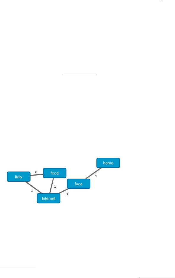
Figure 2: Example of computation of weighted Jaccard dis-
tance.
Example 1. We give a sample of computation of
the weighted Jaccard distance referring to Figure 2.
Here, the weighted neighbourhood N(Internet) of In-
ternet is
{(italy,1),( f ood,1),( f ace,3),(Internet,3)},
6
A multiset is a set where an element can recur more
than once, and can be defined as a set of couples (element,
multiplicity) (Aigner, 2012).
that of home is
{( f ace,1),(home,1)}.
Then we will have that N(Internet) ∪ N(home) corre-
sponds to
{(italy,1),( f ood,1),( f ace,3),(Internet,3),(home,1)},
with cardinality 9, and
N(Internet) ∩ N(home) = {( f ace,1)},
whose cardinality is 1. This means that the
distance d
J
(Internet,home) in our sample graph
is 1 −
1
9
= 0,888 . . . We could similarly obtain
d
J
(Internet, f ood) = 0,4 and d
J
(italy,home) = 1. The
latter result is evident, since there are no common
neighbours between the two words.
The weighted Jaccard distance we defined in
Equation 2 just considers all the elements in the
neighbourhood of a node v. Of course, it could be ex-
panded to neighbourhoods of depth greater than 1: for
increasing depths, we would take into account neigh-
bourhoods of neighbour words of v, neighbourhoods
of neighbourhoods, and so on, depending on the cho-
sen depth. This means that, increasing the depth, at
some threshold the Jaccard distance will begin losing
significance. In this work we decided to consider the
case of degree 1.
Now, using the distance defined in Equation 2, we
can define the word metric space
7
W
F
= (V
F
, d
J
) de-
rived from graph F. Having a metric space allows
us to employ aggregative clustering techniques, like
e.g. k-medoids, as will be shown in the following
Sections.
We shall content ourselves by remarking that W
F
is a bounded space (the maximum distance between
any two points is 1) and that we know that the dis-
tance between any two points v and w is less than 1
if and only if there is a path of length at most 2 con-
necting them in F. Indeed, it is quite difficult, if not
outright impossible, to visualize the (discrete) metric
space W
F
: even if it were of Euclidean nature, the
problem of retrieving its underlying structure from its
elements and the distance still remains an open area
of research in Mathematics, called Distance Geome-
try (Mucherino et al., 2012).
3 THE CLUSTERING
ALGORITHM
Given a data set of tweets, we construct the global
graph G from it, as defined in Section 2.3. We choose
7
For detailed definitions, see (Rudin, 1964).
Word Sense Discrimination on Tweets: A Graph-based Approach
141
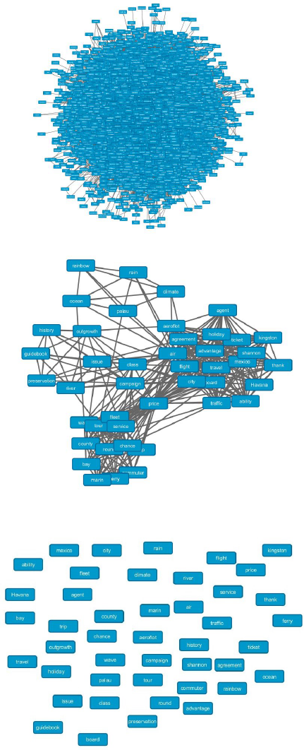
(a) First we build the global word graph.
(b) Then, we take the subgraph induced by the open neigh-
bourhood of a given term, e.g. tourist.
(c) Finally, we obtain a metric space of words, where we
know the distance between any two terms.
Figure 3: Progression from word graph to word metric
space.
a term v whose senses we want to discriminate and the
corresponding metric space W
G
v
= (V
G
v
,d
J
) derived
from its word cloud G
v
(see Sections 2.3 and 2.4).
Our goal is to find a partition C
v
= {C
1
, . . . ,C
k
v
} of
W
G
v
, with the assumption that each C
i
will implicitly
define one of the k
v
senses that v assumes in the tweets
we are considering.
The number k
v
of clusters is not pre-determined.
However, we expect every term we want to disam-
biguate to give rise to one or two bigger clusters and
a host of smaller ones: it is a common pattern for an
ambiguous word to have a more used sense and many
rarer ones. The clustering process starts by select-
ing the word u ∈ V
G
v
with highest degree in G
v
as the
representative of the first cluster. According to this
choice, u can be viewed as a possible “sense hub”,
i.e. a central word around which many others tend to
gravitate and which could possibly be the most im-
portant representant of one of v’s senses. We set u
as the medoid of the cluster. We then check the dis-
tance between u and each other word w in W
G
v
. If u
and w are close enough, i.e. the distance is less than
or equal to a previously set threshold σ ∈ [0,1), we
add w to u’s cluster. Otherwise, if w is more distant
than σ, w will originate a new cluster. This iterative
process will be applied to all words w ∈ W
G
v
. Once
all the words have been processed, at the end of the
first iteration we will have obtained k
v
clusters, each
represented by a medoid. Now, for each cluster the
corresponding medoid, i.e. the element with lowest
mean distance from all the other elements in the clus-
ter, will be updated. Then, we will start the next it-
eration, again (re)assigning every word to the cluster
whose medoid it is closest to. We repeat the whole
process until convergence is reached, i.e. until either
the medoids do not change between consecutive iter-
ations, or a maximum number of iterations are per-
formed. At the end of the clustering process, the par-
titioning C
v
= {C
1
, . . . ,C
k
v
} will be identified with all
the possible senses that can be associated to the word
v in the tweets.
Given a threshold σ and a maximum number of
iterations maxiter, the proposed algorithm works as
displayed in Algorithm 1. By C
x
we will denote the
cluster represented by its medoid x.
Labelling
Finally, after having obtained the clustering
C
v
= {C
1
, . . . ,C
k
v
} relative to the chosen term v,
we want to use the C
i
’s to label each of v’s occur-
rences in the tweets. We adopt a sort of majority
voting system: for each reduced tweet where v
appears, we compute the Jaccard distance between
that tweet’s set of words T = {t
1
, . . . ,t
n
} and each
cluster C
i
. Then, we assign to the term the label
referring to the cluster
KDIR 2015 - 7th International Conference on Knowledge Discovery and Information Retrieval
142

Algorithm 1: Aggregative algorithm (σ, maxiter).
1: C = {} The set of clusters
2: M = M
0
= {} The sets of new and old of medoids
3: u = argmax
w∈G
v
deg(w)
4: M = M ∪ u
5: C
u
= {}
6: C = C ∪C
u
7: numiter = 0
8: do
9: M = M
0
10: for w ∈ W
G
v
do
11: if ∃m ∈ M | d
J
(w,m) < σ then
12: x = arg min
m∈M
d
J
(w,m)
13: C
x
= C
x
∪ w
14: else
15: M = M ∪ w
16: C
w
= {w} w originates a new cluster
17: C = C ∪C
w
18: end if
19: end for
20: M
0
= {}
21: for m ∈ M do Medoid recalculation
22: m
0
= argmin
µ∈C
m
∑
w∈C
m
d
J
(µ,w)
23: M
0
= M
0
∪ m
0
24: end for
25: numiter = numiter + 1
26: while M 6= M
0
and numiter ≤ maxiter
27: return C
C
min
= argmin
C∈C
v
, (3)
i.e. the cluster closest to T in terms of Jaccard dis-
tance. It is possible that not every cluster will be as-
signed to a term’s occurrence; these are “weak” clus-
ters that are maybe either too insignificant or too fine-
grained. In any case, we have thus defined a mapping
l that goes from the set T
v
of tweets in which v occurs
to the clusters in C
v
.
4 RESULTS AND EVALUATIONS
In order to evaluate the performances of our proposed
approach from a quantitative point of view, we have
created a benchmark data set consisting of tweets. We
are going to present, evaluate and discuss the results
obtained on it by our algorithm. We are also go-
ing to compare it with another clustering algorithm
called Chinese Whispers (Biemann, 2006). Finally,
we are going to evaluate our algorithm also on an of-
ficially recognized data set such as that of Task 14 at
SemEval-2010 (Manandhar et al., 2010), noting that
its nature is quite different from our tweet data set.
4.1 The Tweet Data Set
The data set we decided to examine consisted of 5291
tweets in English, downloaded from Twitter on a sin-
gle day using eleven different keywords, averaging
about 500 tweets per keyword. Keywords were cho-
sen to be common words that may possess many dif-
ferent senses (see Table 1). We are taking into ac-
count only nouns and not verbs, to avoid complicat-
ing issues related to the many conjugated and some-
times irregular forms verbs can assume. Every tweet
contains one of our keywords as a free-standing term
(e.g. a hashtag like #milanfashion would not count as
an instance of milan).
The terms that we want to disambiguate corre-
spond to the keywords used in the creation of our
benchmark. To this purpose, we have manually dis-
ambiguated them. To briefly illustrate our criteria, let
us consider e.g. the keyword mcdonald: we made
a distinction between each single individual bearing
this name, the fast food restaurants as a whole, and the
company. Of course, many other possible senses exist
for mcdonald. A problem arises with complex expres-
sions we might call collocations
8
: there, we decided
to give a term the sense of the entire collocation if it
appears as the head of its noun phrase (as in “Mars
Hill”, a place name) or if it is part of a fixed proper
name (as in “Thirty seconds to Mars”, a band name).
If the term is a complement, we assign to it its “basic”
sense (in “Inter Milan”, the football team, milan will
be tagged as the city).
To run our algorithm on the tweets, we first have to
pre-process them. Tweets are lowercased, tokenized
and their parts of speech tagged using the ARK POS
tagger for Twitter. Then, we proceed with word filter-
ing, as explained in Section 2.2.
After pre-processing, we can build the global co-
occurrence word graph G, as detailed in Section 2.3.
In this specific case, G will consist of 12439 nodes or
distinct words and 145256 edges. Its average short-
est path has a length of 2,738 and its average clus-
tering coefficient is 0,78. Clearly, G is warped by
construction around our eleven keywords, which are
the elements with the highest degrees. This serves
our purpose to test our algorithm in a controlled envi-
ronment where we know at which “most ambiguous”
terms we have to direct our attention. Even so, this
is not far from the realistic assumption that the terms
whose disambiguation is most relevant are the most
preeminent ones in a co-occurrence graph in terms of
degree and other coefficients.
4.2 Evaluation Methods
We used two evaluation methods: the first one was
defined by us as a way to assess the quality and co-
8
See chapter 5 of (Manning and Sch
¨
utze, 1999)
Word Sense Discrimination on Tweets: A Graph-based Approach
143

Table 1: Keywords and entities.
Keywords Tagged
tweets
No. of
senses
Most common senses (≥ 10%)
blizzard 463 23 snowstorm 43%, video game company 37%
caterpillar 467 23 CAT machines 30%, animal 24%, The Very Hungry Caterpillar 17%, CAT
company 16%
england 474 11 country (UK) 65%, national football team 10%, New England (USA) 10%
ford 558 12 Harrison Ford 40%, Ford vehicles 30%, Tom Ford (fashion designer) 25%
india 474 5 country 50%, national cricket team 48%
jfk 474 13 New York airport 61%, John Fitzgerald Kennedy 33%
mcdonald 425 47 McDonald’s (restaurants) 38% , McDonald’s (company) 31%
mars 440 24 planet 66%, Bruno Mars 17%
milan 594 41 Milano (Italy) 58%, A.C. Milan football team 24%
pitbull 440 7 rapper 49%, dog breed 48%
venice 482 9 Venezia (Italy) 55%, Venice beach (California) 42%
herence of our clusters, while the second one is the
Adjusted Mutual Information score (AMI).
4.2.1 Our Method
In Section 3 we defined the labelling mapping l that
labels a term with the cluster representing one of its
found senses. We want to compare this labelling
with the ground truths arising from our manual an-
notations, as explained in Section 4.1. Similarly to
the construction of l, we define a mapping m that
goes from the clustering C
v
to all the h true senses
G
v
= {g
1
, . . . ,g
h
} of a chosen word v in the following
way: given a cluster C
i
, we compute the Jaccard dis-
tance between the set of all the words appearing in all
the tweets labelled with C
i
(i.e. the contexts of C
i
) and
the set of all the words appearing in all the tweets la-
belled with a true sense g
j
(i.e. the contexts of g
j
), for
each j = 1, . . . ,h. We then assign to C
i
the sense g
j
to
which it is closest. The mapping m is almost always
not bijective, even if this would be the ideal case. We
therefore define the local labelling accuracy score of v
as the ratio of correctly labelled tweets according to m
to the number of tweets where v occurs. Analogously,
a global accuracy score can be computed.
4.2.2 Adjusted Mutual Information
Adjusted Mutual Information was introduced after the
more classical measures of F-score and V-measure,
used for the evaluation of task 14 at SemEval-2010,
detailed in (Manandhar et al., 2010), were found to
be biased, depending too much just on the number
of clusters: the more clusters, the higher the F-score
and the lower the V-measure (to a minimum of 0 if
just one cluster was detected for a specific term), and
viceversa for a low number of clusters, apparently re-
gardless of their quality. It was probably for this rea-
son that the best results were achieved by the base-
line algorithm that assigns to a word its most frequent
sense. Adjusted Mutual Information was introduced
to circumvent this problem, taking into account the
fact that two big clusterings tend to have a higher mu-
tual information score, even if they do not truly share
more information (Vinh et al., 2009).
4.3 Results
In Table 2 local accuracy scores relative to our key-
words for our aggregative clustering algorithm with
different σ thresholds and the Chinese Whispers al-
gorithm are shown. Only values greater than 0,9 are
shown for σ, since this is where the overall most sig-
nificant scores were achieved.
Looking at Table 2, we see that the keywords with
more dispersed senses (i.e. caterpillar, mcdonald)
tend to have the lowest accuracies, whereas more po-
larized (i.e. pitbull, venice) words give better results.
By “polarized” and “dispersed” we denote a word
whose two main senses, as from Table 1, cover re-
spectively more or less than 90% of the tweets where
it occurs. Interestingly, this behaviour is not exactly
mirrored by the number of found clusters. Of course,
the number of clusters tends to diminish as the thresh-
old increases, since a greater σ means that the algo-
rithm is more permissive, in the sense that clusters
have a bigger radius and contain more words. On
the contrary, the Chinese Whispers algorithm finds
a very low number of clusters, probably because of
the small-world nature of the underlying graph: since
this algorithm assigns to a node a sense based on the
senses of its neighbours, a couple of hub nodes (as
mentioned in Section 2.3) will tend to influence most
of the other nodes in the graph. In the light of this,
Chinese Whispers will closely resemble the “most fre-
quent sense” baseline algorithm. This behaviour im-
KDIR 2015 - 7th International Conference on Knowledge Discovery and Information Retrieval
144
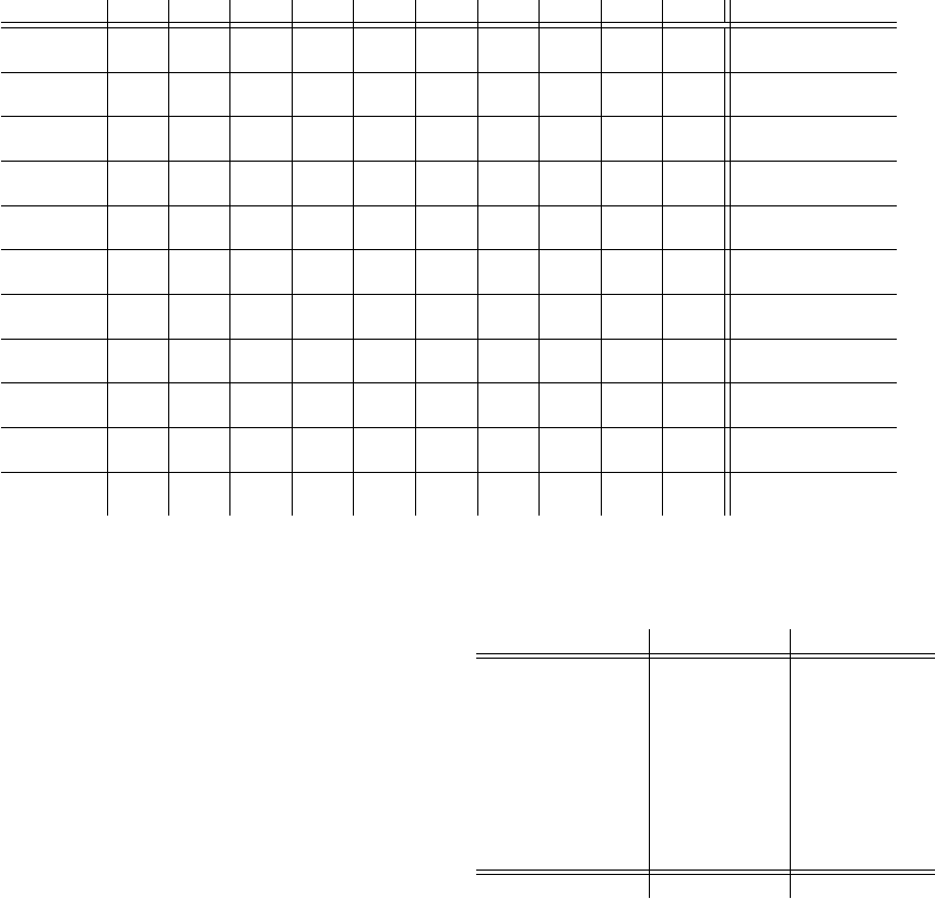
Table 2: Local accuracies (in percentages, first row) and number of clusters for each keyword.
σ = 0,9 0,91 0,92 0,93 0,94 0,95 0,96 0,97 0,98 0,99 Chinese Whispers
blizzard 59,8 55,1 57,5 50,8 53,1 53,3 54,4 47,3 47,3 45,1 43,0
47 43 38 35 27 24 16 12 12 6 1
caterpillar 42,4 41,3 42,6 42,8 42,4 43,7 30,6 42,8 43,7 39,0 43,7
31 29 26 21 20 14 10 9 7 6 6
england 40,5 40,5 41,8 53,6 60,5 63,3 63,5 65,4 65,4 65,2 65,4
57 49 48 36 30 25 21 15 14 9 1
ford 74,2 82,3 71,3 78,3 63,3 72,2 74,7 81,9 39,6 39,6 80,1
22 18 19 15 13 10 6 6 4 3 3
india 70,3 67,1 77 71,1 76,8 79,5 82,1 82,9 70,3 77,0 63,1
61 53 44 43 35 30 24 20 18 16 2
jfk 64,8 72,6 63,5 67,3 68,4 69,4 70,7 67,1 69,8 78,1 61,2
30 30 28 24 22 17 14 11 10 8 2
mcdonald 44,7 40,2 41,9 40,5 44,2 44,7 40,2 46,4 44,9 37,9 40,7
36 35 30 26 23 20 18 13 11 10 3
mars 74,1 65,5 64,8 74,5 73,4 78,9 68,0 80 66,0 68,0 66,4
17 13 11 8 8 6 6 4 4 3 2
milan 53,7 54,0 51,0 57,2 62,8 58,2 56,7 58,8 56,2 50,2 58,2
45 42 40 34 27 21 23 16 15 14 1
pitbull 70 64,8 65,9 59,8 76,3 75,7 52,5 76,6 75 51,6 81,1
46 37 36 33 26 23 15 11 10 7 3
venice 72,6 69,9 67,8 78,0 76,8 63,5 79,5 71,6 64,3 82,4 55,0
38 31 28 25 24 20 16 14 10 8 1
plies too simplistic results that are in contrast with the
variety of possible and actual senses for each term,
as highlighted in Table 1. In this sense, the Chinese
Whispers algorithm fails to capture all the facets of a
term.
The algorithm we proposed generally has better
performances than Chinese Whispers, especially for
the threshold 0,97. In that case, the respective global
accuracies are 69,6% and 60,1%. The same trend can
be observed in Table 3 when applying the Adjusted
Mutual Information score, both on our data set and
on SemEval-2010’s task 14’s data set for nouns. It is
to be noticed that the scores are much lower on Se-
mEval’s data set, probably due to the fact that it is
much sparser than ours. In fact, disambiguation is
done for 50 terms, whose number of text samples can
vary between few dozens and nearly one thousand,
and the samples themselves come from very differ-
ent media and sources. As a consequence, a method
like the one we proposed will have to work on much
less significant contexts and word graphs, leading to
a more fragmented clustering. Nonetheless, our algo-
rithm still outperforms Chinese Whispers and is not
far from the best results achieved during SemEval
2010’s competition.
5 CONCLUSION
In this paper we presented an unsupervised, graph-
based approach to Word Sense Discrimination. Our
Table 3: Compared overall AMI scores for the aggregative
clustering algorithm and for Chinese Whispers on our tweet
data set and on SemEval-2010’s task 14 data set.
Tweet data set SemEval-2010
σ = 0,91 0,162 0,048
σ = 0,92 0,161 0,046
σ = 0,93 0,178 0,043
σ = 0,94 0,175 0,045
σ = 0,95 0,188 0,040
σ = 0,96 0,193 0,037
σ = 0,97 0,209 0,037
σ = 0,98 0,192 0,036
σ = 0,99 0,196 0,032
Chinese Whispers 0,116 0,013
aim was to discriminate terms in spontaneous and un-
controlled texts, so that we chose to focus on tweets.
The main challenge we encountered was the diffi-
culty of handling a large graph of the small-world
type: even after word filtering, the graph structure
that arises from a text could be still considered very
noisy. In the end, defining a distance on the graph,
we resolved to “loosen” the graph into a metric space,
where it is possible to apply well known methods such
as the aggregative clustering algorithm we proposed,
which yields good results.
Apart from the design of the algorithm itself,
we have to underline that word clustering represents
just the last step of a procedure that starts with pre-
processing and tokenization of a text, which are both
mostly supervised in nature and have a fundamental
influence on the outcomes of the algorithm. Further-
Word Sense Discrimination on Tweets: A Graph-based Approach
145
more, text pre-processing poses many challenges for
languages of a different typology and with richer mor-
phology than English. For these reasons, we envision
as our possible future goals to further investigate re-
lations between text pre-processing and clustering re-
sults and how to make the whole process as unsuper-
vised and language-independent as possible.
REFERENCES
Aigner, M. (2012). Combinatorial theory, volume 234.
Springer Science & Business Media.
Biemann, C. (2006). Chinese whispers: an efficient graph
clustering algorithm and its application to natural lan-
guage processing problems. In Proceedings of the first
workshop on graph based methods for natural lan-
guage processing, pages 73–80. Association for Com-
putational Linguistics.
Brody, S. and Lapata, M. (2009). Bayesian word sense in-
duction. In Proceedings of the 12th Conference of
the European Chapter of the Association for Compu-
tational Linguistics, pages 103–111. Association for
Computational Linguistics.
Dorow, B. and Widdows, D. (2003). Discovering corpus-
specific word senses. In Proceedings of the tenth
conference on European chapter of the Association
for Computational Linguistics-Volume 2, pages 79–
82. Association for Computational Linguistics.
Fritsch, R. and Piccinini, R. (1990). Cellular structures in
topology, volume 19. Cambridge University Press.
G
¨
ardenfors, P. (2004). Conceptual spaces: The geometry of
thought. MIT press.
Hope, D. and Keller, B. (2013). Maxmax: a graph-based
soft clustering algorithm applied to word sense induc-
tion. In Computational Linguistics and Intelligent Text
Processing, pages 368–381. Springer.
i Cancho, R. F. and Sol
´
e, R. V. (2001). The small
world of human language. Proceedings of the Royal
Society of London. Series B: Biological Sciences,
268(1482):2261–2265.
Lin, D. (1998). Automatic retrieval and clustering of sim-
ilar words. In Proceedings of the 36th Annual Meet-
ing of the Association for Computational Linguistics
and 17th International Conference on Computational
Linguistics-Volume 2, pages 768–774. Association for
Computational Linguistics.
Manandhar, S., Klapaftis, I. P., Dligach, D., and Pradhan,
S. S. (2010). Semeval-2010 task 14: Word sense in-
duction & disambiguation. In Proceedings of the 5th
international workshop on semantic evaluation, pages
63–68. Association for Computational Linguistics.
Manning, C. D. and Sch
¨
utze, H. (1999). Foundations of
statistical natural language processing. MIT press.
Mihalcea, R. and Faruque, E. (2004). Senselearner: Min-
imally supervised word sense disambiguation for all
words in open text. In Proceedings of ACL/SIGLEX
Senseval, volume 3, pages 155–158.
Mucherino, A., Lavor, C., Liberti, L., and Maculan, N.
(2012). Distance geometry: theory, methods, and ap-
plications. Springer Science & Business Media.
Navigli, R. (2009). Word sense disambiguation: A survey.
ACM Computing Surveys (CSUR), 41(2):10.
Navigli, R. (2012). A quick tour of word sense disambigua-
tion, induction and related approaches. In SOFSEM
2012: Theory and practice of computer science, pages
115–129. Springer.
Navigli, R. and Ponzetto, S. P. (2012). Babelnet: The au-
tomatic construction, evaluation and application of a
wide-coverage multilingual semantic network. Artifi-
cial Intelligence, 193:217–250.
Owoputi, O., O’Connor, B., Dyer, C., Gimpel, K., Schnei-
der, N., and Smith, N. A. (2013). Improved part-
of-speech tagging for online conversational text with
word clusters. In HLT-NAACL, pages 380–390.
Rudin, W. (1964). Principles of mathematical analysis, vol-
ume 3. McGraw-Hill New York.
Schmitz, M., Bart, R., Soderland, S., Etzioni, O., et al.
(2012). Open language learning for information ex-
traction. In Proceedings of the 2012 Joint Conference
on Empirical Methods in Natural Language Process-
ing and Computational Natural Language Learning,
pages 523–534. Association for Computational Lin-
guistics.
Sch
¨
utze, H. (1998). Automatic word sense discrimination.
Computational linguistics, 24(1):97–123.
V
´
eronis, J. (2004). Hyperlex: lexical cartography for in-
formation retrieval. Computer Speech & Language,
18(3):223–252.
Vinh, N. X., Epps, J., and Bailey, J. (2009). Information
theoretic measures for clusterings comparison: is a
correction for chance necessary? In Proceedings of
the 26th Annual International Conference on Machine
Learning, pages 1073–1080. ACM.
Watts, D. J. and Strogatz, S. H. (1998). Collective dynamics
of small-worldnetworks. nature, 393(6684):440–442.
Widdows, D. and Dorow, B. (2002). A graph model for
unsupervised lexical acquisition. In Proceedings of
the 19th international conference on Computational
linguistics-Volume 1, pages 1–7. Association for Com-
putational Linguistics.
Zhong, Z. and Ng, H. T. (2010). It makes sense: A
wide-coverage word sense disambiguation system for
free text. In Proceedings of the ACL 2010 System
Demonstrations, pages 78–83. Association for Com-
putational Linguistics.
KDIR 2015 - 7th International Conference on Knowledge Discovery and Information Retrieval
146
