Clustering using Cellular Genetic Algorithms

Nuno Leite

1,3

, Fernando Mel

ıcio

and Agostinho C. Rosa

2,3

Instituto Superior de Engenharia de Lisboa/ADEETC, Polytechnic Institute of Lisbon, Rua Conselheiro Em

ıdio Navarro,

n.° 1, 1959-007, Lisboa, Portugal

Department of Bioengineering/Instituto Superior T

ecnico, Universidade de Lisboa, Av. Rovisco Pais, n.° 1, 1049-001,

Lisboa, Portugal

Institute for Systems and Robotics/LaSEEB, Instituto Superior T

ecnico, Universidade de Lisboa, Av. Rovisco Pais, n.° 1,

TN 6.21, 1049-001, Lisboa, Portugal

Keywords:

Cellular Genetic Algorithms, Clustering, Classiﬁcation, Evolutionary Computation, Nature Inspired

Algorithms.

Abstract:

The goal of the clustering process is to ﬁnd groups of similar patterns in multidimensional data. In this work,

the clustering problem is approached using cellular genetic algorithms. The population structure adopted in

the cellular genetic algorithm contributes to the population genetic diversity preventing the premature con-

vergence to local optima. The performance of the proposed algorithm is evaluated on 13 test databases. An

extension to the basic algorithm was also investigated to handle instances containing non-linearly separable

data. The algorithm is compared with nine non-evolutionary classiﬁcation techniques from the literature, and

also compared with three nature inspired methodologies, namely Particle Swarm Optimization, Artiﬁcial Bee

Colony, and the Fireﬂy Algorithm. The cellular genetic algorithm attains the best result on a test database. A

statistical ranking of the compared methods was made, and the proposed algorithm is ranked ﬁfth overall.

1 INTRODUCTION

Clustering is an important unsupervised learning ap-

proach used in applications in areas such as data min-

ing, statistical data analysis, data compression, or vec-

tor quantization. The task of clustering is to discover

natural groupings of a set of patterns, points, or ob-

jects (Jain, 2010).

Clustering approaches are generally categorized

into two classes (Jain, 2010): hierarchical and par-

titional. In hierarchical clustering, nested clusters are

found recursively according to two modes, agglomer-

ative and divisive. In the agglomerative mode, the

clustering process starts with each data point in its

own cluster and then proceeds merging the most sim-

ilar pair of clusters successively to form a cluster hi-

erarchy. In the divisive (top-down) mode, the clus-

tering starts with all the data points in one cluster

and then proceeds by recursively dividing each cluster

into smaller clusters. Partitional clustering algorithms

work differently compared to hierarchical clustering

algorithms as they ﬁnd all the clusters at the same

time as a partition of the data without imposing a hi-

erarchical structure. The prototype-based clustering

algorithms are the most popular partitional clustering

algorithms. In these, each cluster is represented by

its center and the objective function used is the sum

of squared distances of the data points to the cluster

centers they are assigned to (Mirkin, 1996; Borgelt,

2006). An example of a partitional clustering algo-

rithm is the popular k–means algorithm. Although

still widely used, the main drawback of the k–means

algorithm is that it converges to a local minima from

the starting position of the search (Selim and Ismail,

1984).

The clustering process can be done through two

ways: by unsupervised learning or by supervised

learning. In unsupervised clustering, also called au-

tomatic clustering, there’s no information about the

classes of the patterns, and the clustering is done by

ﬁnding the natural aggregations in the dataset. On

the other way, in supervised clustering, also known

as classiﬁcation, a classiﬁer is learned given a train-

ing set with known pattern classes. After the training

phase, a test set is classiﬁed based on the learned clas-

siﬁer. The learned classiﬁer contains information of

the optimal cluster centers that characterize the parti-

tions in the training set. These cluster centers are used

to classify the patterns in the test set.

In the recent years, nature inspired algorithms

366

Leite, N., Melício, F. and Rosa, A..

Clustering using Cellular Genetic Algorithms.

In Proceedings of the 7th International Joint Conference on Computational Intelligence (IJCCI 2015) - Volume 1: ECTA, pages 366-373

ISBN: 978-989-758-157-1

have been proposed to solve clustering and classi-

ﬁcation problems. Examples include Genetic Al-

gorithms (Falkenauer, 1998; Maulik et al., 2000),

Memetic Algorithms (Ni et al., 2013), Artiﬁcial Bee

Colony (ABC) (Karaboga and Ozturk, 2011), Parti-

cle Swarm Optimization (PSO) (Falco et al., 2007),

Fireﬂy Algorithm (FA) (Senthilnath et al., 2011), and

Cuckoo Search Algorithm (Zhao et al., 2014). Re-

cently, hybrid evolutionary algorithms which com-

bine evolutionary algorithms with the k–means algo-

rithm were also proposed (Niknam and Amiri, 2010).

In the study presented in this work, a novel ap-

proach of cellular genetic algorithms (cGA) (Alba

and Dorronsoro, 2008) is proposed for solving the

clustering problem. The cGA is based on the par-

allel cellular model which maintains a greater pop-

ulation diversity compared to the standard evolution-

ary algorithm, thus contributing to ﬁnd solutions with

better quality (Alba and Dorronsoro, 2008). To the

extent of our knowledge, cellular evolutionary algo-

rithms have not yet been applied successfully to the

clustering problem. The cGA is applied to classiﬁca-

tion benchmark problems on 13 typical test databases.

The cGA is compared with nine non-evolutionary

classiﬁcation techniques from the literature, and also

compared with three nature inspired methodologies,

namely PSO (Falco et al., 2007), ABC (Karaboga and

Ozturk, 2011), and the FA (Senthilnath et al., 2011).

The remaining of the paper is organized as fol-

lows. In Section 2, the clustering problem is formally

deﬁned. Section 3 presents the canonical cellular evo-

lutionary algorithm. In Section 4, the adaptation of

the cGA for classiﬁcation is described. Section 5 re-

ports the experimental results. Some conclusions are

drawn in Section 6.

2 CLUSTERING AND

CLASSIFICATION PROBLEMS

Given a set of multidimensional data, the clustering

process consists in ﬁnding groups of patterns, or clus-

ters, in the data whose members are more similar to

each other than they are to other patterns (Duda et al.,

2000). The clustering is done based on some simi-

larity measure (Jain et al., 1999), where the measure

based on the distance is generally used.

The clustering problem can be stated as an opti-

mization problem, as in (Marinakis et al., 2008). In

order to formulate the clustering problem the follow-

ing symbols were deﬁned:

• K, is the number of clusters.

• N, is the number of objects.

• x

∈ R

,(i = 1, . . . , N) is the location of the ith

pattern.

• z

∈ R

,( j = 1, . . . , K) is the center of the jth clus-

ter, computed as:

∑

∈C

(1)

where N

is the number of objects in the jth cluster

denoted by C

The optimization problem is formulated as:

Minimise J(w, z) =

∑

i=1

∑

j=1

i j

k x

− z

(2)

Subject to

∑

j=1

i j

= 1, i = 1,. . . , N (3)

i j

= 0 or 1, i = 1,. . . , N, j = 1,. . . , K. (4)

In Eq. (1), each z

cluster center is computed as the

centroid of the region formed by the cluster objects.

The goal of the clustering problem, as given in Eq. (2),

is to ﬁnd the clusters centers z

, such that the sum of

the squared Euclidean distances between each pattern

and the center of its cluster is minimized.

As mentioned in the introduction, the related

problem known as classiﬁcation is solved in this

work. To assess the quality of the classiﬁcation, the

performance measure – classiﬁcation error percentage

(CEP) – was used:

CEP = 100 ·

Number of misclassiﬁed instances

Total size of test set

(5)

3 CELLULAR GENETIC

ALGORITHMS

The cellular evolutionary algorithm (cGA) used to

solve the Clustering problem relies on the parallel

cellular model. In this model, the populations are

organized in a special structure deﬁned as a con-

nected graph, in which each vertex is a solution that

communicates with its neighbours (Alba and Dor-

ronsoro, 2008). More speciﬁcally, individuals are set

in a toroidal mesh and are only allowed to recombine

with the close neighbours (Figure 1). The population

structure used in cellular evolutionary algorithms con-

tributes to the population genetic diversity thus avoid-

ing the premature convergence to a local optimum.

Algorithm 1 depicts the steps of the general cel-

lular genetic algorithm. First, the initial population is

Clustering using Cellular Genetic Algorithms

367

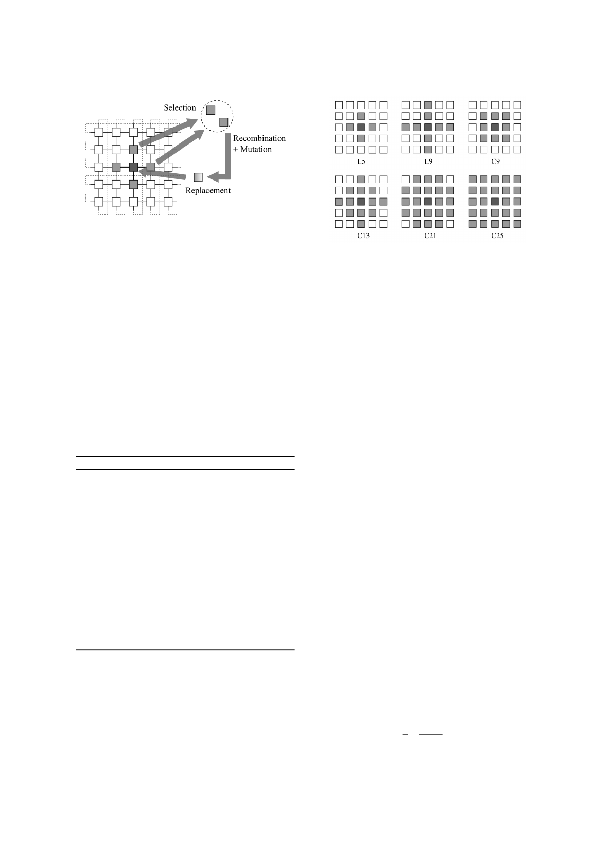
Figure 1: The parallel cellular model for evolutionary algo-

rithms.

generated and evaluated. Then, while the stop condi-

tion is not achieved (e.g., maximum number of itera-

tions is achieved, ﬁtness value of the best individual

is within a desired interval), the following steps are

executed sequentially for each population’s individ-

ual: (1) obtain the individual’s neighbours according

to a speciﬁed neighbourhood, (2) select individuals

to recombine from the neighbours’ set, (3) recombine

(crossover and mutation) the selected offspring, and

(4) put the best offspring in an auxiliary population.

After doing steps (1) to (4) for all the elements of

the population, the auxiliary population replaces the

original population. In this version of the cGA, all the

individuals are updated at the same time, so the the

algorithm is called synchronous cGA. Figure 2 illus-

trates six typical neighbourhoods used in the cGA.

Algorithm 1: Pseudo-code of the canonical cGA.

1: procedure CGA(cga) // Parameters in ‘cga’

2: GenerateInitialPopulation(cga.pop);

3: Evaluation(cga.pop);

4: while !StopCondition() do

5: for indiv ← 1 to cga.popSize do

6: neighs ← GetNeighs(cga, pos(indiv));

7: par ← Selection(neighs);

8: offs ← Recombination(cga.P

, par);

9: offs ← Mutation(cga.P

, offs);

10: Evaluation(offs);

11: Replace(pos(indiv), offs, auxPop);

12: end for

13: cga.pop ← auxPop;

14: end while

15: end procedure

In the implemented approach, it was used the L5

neighbourhood type, also known as the von Neu-

mann neighbourhood. This neighbourhood promotes

a smother actualisation of the populations compared

with the other neighbourhoods. In the selection pro-

cedure (Figure 1), one of the four neighbours of the

central individual is selected with a binary tourna-

Figure 2: Typical neighbourhoods used in cellular evolu-

tionary algorithms.

ment. The chosen neighbour and the middle individ-

ual are then recombined producing two offspring so-

lutions. A mutation operator is then applied to these

two solutions and the best offspring is selected. The

offspring solution is compared with the original in-

dividual, and, if it is better, it will replace the origi-

nal solution. Otherwise, the original solution is main-

tained.

4 CGA APPLIED TO

CLASSIFICATION

In this section, the cGA adaptation to tackle classiﬁ-

cation problems is described.

4.1 Encoding

Given an instance with C classes and N attributes, the

classiﬁcation problem considered consists in ﬁnding

the optimal positions of the C centroids in the N-

dimensional space. The i-th individual of the popu-

lation is encoded as follows:

(~p

,...,~p

) (6)

where the j-th centroid position is formed by N

real numbers representing the coordinates in the N-

dimensional space (Falco et al., 2007):

= {p

1,i

,..., p

N,i

}. (7)

So, each population individual is composed by C ∗ N

components, each represented by a real number.

4.2 Fitness Function

Each solution i is evaluated using the weighted ﬁtness

function ψ

(i) from (Falco et al., 2007):

(i) =



(i)

100.0

+ ψ

(i)



, (8)

ECTA 2015 - 7th International Conference on Evolutionary Computation Theory and Applications

368

where ψ

(i) is given by

(i) =

100.0

Train

∑

j=1

δ(~x

) (9)

δ(~x

) =



1 if CL(~x

) 6= CL

known

(~x

0 otherwise.

(10)

and ψ

(i) is given by

(i) =

Train

∑

j=1



,~p

known

(~x

)



. (11)

As described in (Falco et al., 2007), the function ψ

(i)

is computed in two steps. In the ﬁrst step, the train-

ing set patterns are assigned to the class of the closest

centroid in the N-dimensional space. Then, the ﬁtness

of the i-th individual is computed as the percentage

of incorrectly assigned instances on the training set,

i.e., counts the number of patterns ~x

for which the

assigned class CL(~x

) is different from the true class

known

(~x

). The function ψ

(i) is computed in one

step as the sum of the Euclidean distances between

each pattern ~x

in the training set and the centroid of

the true cluster (~p

known

(~x

)

When computing the distance, the components of

the i-th individual are normalized using the Min-Max

Normalization.

4.3 Population Initialization

The components of each individual in the population

are initialized with random numbers in the range [0,1]

generated with uniform distribution. Notice that the

components could have been initialized with any ran-

dom numbers, or even with the components of ran-

dom chosen patterns. Empirical tests were undertaken

with different ranges ([0, 1], [0,5], [0, 50], and com-

ponents of random patterns). The results showed that

there are not signiﬁcant differences between the meth-

ods.

4.4 Crossover

Given two parent solutions, the crossover recombina-

tion process exchanges, in a probabilistic fashion, the

information between the parent chromosomes pro-

ducing two offspring chromosomes. In this work,

single-point crossover with crossover probability P

was used.

4.5 Mutation

The mutation operator used was based on that pub-

lished in (Maulik et al., 2000). For a ﬁxed probability

Table 1: Properties of the examined databases.

N D C miss

Balance 4 625 3 No

Credit 15 690 2 Yes

Dermatology 34 366 6 Yes

Diabetes 8 768 2 No

E.Coli 7 327 5 No

Glass 9 214 6 No

Heart 13 303 2 Yes

Horse Colic 27 368 2 Yes

Iris 4 150 3 No

Thyroid 5 215 3 No

WDBCancer 30 569 2 No

WDBCancer-Int 9 699 2 Yes

Wine 13 178 3 No

, a gene is selected randomly. A number δ in the

range [−1, 1] is generated with uniform distribution.

If the value at a gene position is v, after mutation it

becomes

v =



v · (1 + 2 · δ), v 6= 0,

v + 2 · δ, v = 0.

(12)

With this mutation, the value of the selected gene, v,

is increased or decreased in small random amounts.

4.6 Handling Non-linearly Separable

Problems

As pointed out by De Falco et al. (Falco et al., 2007)

in their work, the use of centroids to approach the

classiﬁcation problem is not adequate in some situ-

ations. The authors list three cases in which an algo-

rithm based on the concept of centroids and distance

to separate the samples into the correct classes is very

difﬁcult or even impossible. The ﬁrst one is when in-

stances of a class are located in two distinct regions

of the N-dimensional space, and these instances are

separated by instances of a second class. The second

situation occurs when a region comprising instances

of a class are completely surrounded by a region con-

taining instances belonging to another class. The third

one is related to the existence of confusion areas in the

search space, i.e., parts of the search space containing

examples belonging to two or more classes. The ﬁrst

two cases could be solved by considering two or more

centroids per class. The third case cannot be solved

effectively with the centroid approach.

To solve the ﬁrst two cases mentioned in the pre-

vious paragraph, the cGA chromosome was extended

by considering K clusters per class (K ≥ 1).

Clustering using Cellular Genetic Algorithms

369

5 EXPERIMENTS AND RESULTS

5.1 Settings

The evaluation of the proposed cGA was carried out

on 13 well known databases taken from the UCI Ma-

chine Learning Repository (Lichman, 2013). The

characteristics of the 13 examined UCI databases are

depicted in Table 1. For each database it is indicated

the number N of attributes composing each instance,

the total instance number D, the number of classes

C into which is divided, and a ﬂag miss indicating

if there is missing data in the database. More in-

formation about the test databases can be obtained

from (Falco et al., 2007).

The algorithm was programmed in the C++ lan-

guage and was based on the ParadisEO frame-

work (Cahon et al., 2004). The experiments were

made on an Intel Core i7-2630QM (CPU @ 2.00 GHz

with 8 GB RAM) PC running Ubuntu 14.04 LTS –

64 bit OS. The Linux kernel used was: 3.13.0-49-

generic. The compiler used was: GCC v. 4.8.2.

In this section, all the statistical tests were per-

formed with a 95% conﬁdence level. The popula-

tion size was set to 100 individuals distributed on a

5 × 20 rectangular grid. The neighbourhood used was

the von Neumann neighbourhood. The crossover and

mutation probabilities, respectively, P

and P

, were

set equal to 0.6 and 0.1. The number of generations

of the cGA was set to 1000.

The parameter values were chosen empirically

taking into account a reasonable balance of obtained

solution quality versus total time taken. The cGA

was executed 20 times on each dataset. The execu-

tion time range from few seconds to about a minute

depending on the dataset size. These times are within

the times published by (Falco et al., 2007).

The source code and the datasets used are

publicly available on the following Git reposi-

tory: https://github.com/nunocsleite/cellularGA-

clustering.

The cGA results were compared with re-

sults produced by nine classical classiﬁcation tech-

niques, and with Particle Swarm Optimization

(PSO) (Falco et al., 2007), Artiﬁcial Bee Colony

(ABC) (Karaboga and Ozturk, 2011), and Fireﬂy Al-

gorithm (FA) (Senthilnath et al., 2011). In order to

perform the classiﬁcation, the datasets were divided

into 75% for training and 25% for testing. The sam-

ples were selected randomly, and divided in a bal-

anced way, in order to guarantee that the percentage of

samples in each class for the testing and training par-

titions was approximately the same. The same trans-

formations to the tested databases as in (Falco et al.,

2007) were carried out (transformation on attributes

with missing data, data shufﬂing, and E.Coli database

class removal).

5.2 Comparison with Other

Classiﬁcation Techniques

Table 2 compares the cGA against three nature based

metaheuristics. Table 3 shows the results of the cGA

on the tested datasets and comparison with the nine

classiﬁcation methods from literature as published

in (Falco et al., 2007). The tables present the aver-

age percentages of incorrect classiﬁcation on the test-

ing set for each algorithm. For every method except

for ABC, the number of runs reported is 20. For the

ABC, the authors report ﬁve runs. From the registered

results it can be observed that the cGA is competitive

with the other techniques, attaining the best value on

the Diabetes dataset.

To assess the effectiveness of the analysed tech-

niques, a statistical ranking was performed (Table 4).

The results of the statistical tests and analysis were

produced using the Java tool of (Garc

ıa and Herrera,

2008). The cGA is positioned in the ﬁfth position.

Relating the metaheuristics, the cGA is superior to

the PSO approach. Relating the other classiﬁcation

methods, only the Bayesian network (Bayes Net) and

the MultiLayer Perceptron Artiﬁcial Neural Network

(MLP ANN) are superior to the cGA.

Table 2: Average percentages of incorrect classiﬁcation on

the testing set. For each test database, the best value ob-

tained among all the techniques is presented in bold.

cGA PSO ABC FA

Balance 12.02 13.12 15.38 14.10

Credit 13.34 18.77 13.37 12.79

Dermatology 4.95 6.08 5.43 5.43

Diabetes 21.61 21.77 22.39 21.88

E.Coli 14.32 13.90 13.41 8.54

Glass 37.36 38.67 41.50 37.74

Heart 18.60 15.73 14.47 13.16

Horse colic 33.91 35.16 38.26 32.97

Iris 1.62 5.26 0.00 0.00

Thyroid 3.49 3.88 3.77 0.00

WDBCancer 4.26 3.49 2.81 1.06

WDBCancer-Int 1.61 2.64 0.00 0.00

Wine 2.84 2.88 0.00 0.00

Figure 3 ilustrates the evolution of the train and

classiﬁcation error as a function of the number of it-

erations for the Balance dataset. Observing Figure 3

it can be concluded that for the Balance dataset the

algorithm steadily improves the training and testing

ECTA 2015 - 7th International Conference on Evolutionary Computation Theory and Applications

370

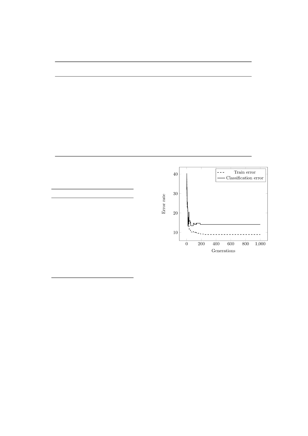
Table 3: Average percentages of incorrect classiﬁcation on the testing set. For each test database, the best value obtained

among all the techniques is presented in bold.

cGA Bayes MLP RBF KStar Bagging Multi NBTree Ridor VFI

Net ANN Boost

Balance 12.02 19.74 9.29 33.61 10.25 14.77 24.20 19.74 20.63 38.85

Credit 13.34 12.13 13.81 43.29 19.18 10.68 12.71 16.18 12.65 16.47

Dermatology 4.95 1.08 3.26 34.66 4.66 3.47 53.26 1.08 7.92 7.60

Diabetes 21.61 25.52 29.16 39.16 34.05 26.87 27.08 25.52 29.31 34.37

E.Coli 14.32 17.07 13.53 24.38 18.29 15.36 31.70 20.73 17.07 17.07

Glass 37.36 29.62 28.51 44.44 17.58 25.36 53.70 24.07 31.66 41.11

Heart 18.60 18.42 19.46 45.25 26.70 20.25 18.42 22.36 22.89 18.42

Horse colic 33.91 30.76 32.19 38.46 35.71 30.32 38.46 31.86 31.86 41.75

Iris 1.62 2.63 0.00 9.99 0.52 0.26 2.63 2.63 0.52 0.00

Thyroid 3.49 6.66 1.85 5.55 13.32 14.62 7.40 11.11 8.51 11.11

WDBCancer 4.26 4.19 2.93 20.27 2.44 4.47 5.59 7.69 6.36 7.34

WDBCancer-Int 1.61 3.42 5.25 8.17 4.57 3.93 5.14 5.71 5.48 5.71

Wine 2.84 0.00 1.33 2.88 3.99 2.66 17.77 2.22 5.10 5.77

Table 4: Average Rankings of the algorithms (higher rank-

ing values are better). The Friedman test on these results

has a p-value of 2.002 × 10

−8

 0.05 making these results

statistically signiﬁcant.

Algorithm Average ranking value

FA 10.58

MLP ANN 9.19

ABC 9.12

Bayes Net 8.81

cGA 8.62

Bagging 8.23

PSO 7.50

KStar 6.35

NBTree 6.31

Ridor 5.62

MultiBoost 4.27

VFI 4.12

RBF 2.31

error in the ﬁrst 30 generations. Then, it suffers from

a slight overﬁtting effect as the train error continues

to decrease and the test error increases.

5.3 Train with Cross-validation

To assess if the results of using a simple split were bi-

ased or not, the classiﬁer was trained using the cross-

validation technique. The instances composing each

dataset were split in the following manner: 75% of

the instances for training the classiﬁer, and 25% for

testing the learned classiﬁer. The training set was fur-

ther divided into a training partition (84%), and a de-

velopment partition (16%). The results for the 13 UCI

Figure 3: Evolution of the train and classiﬁcation error as a

function of the number of iterations for the Balance dataset.

datasets are presented in Table 5. The cross-validation

results are slightly different from those with simple

split but the deviation is not signiﬁcant except for the

Balance and Glass datasets.

5.4 Non-linearly Separable Dataset

In this section, an experiment with a non-linearly

separable synthetic dataset was made. This dataset

(called ‘rings’ (Lourenc¸o et al., 2015)) has N = 450

samples classiﬁed into C = 3 classes (Figure 4). There

are 200 samples of class 1, 200 samples of class 2, and

the remaining 50 samples belong to class 3.

In order classify this dataset a variable number of

clusters per class, instead of a single one, was used.

Figures 5, 6, and 7, illustrate the use of one, three,

and four clusters per class, respectively. As can be ob-

Clustering using Cellular Genetic Algorithms

371

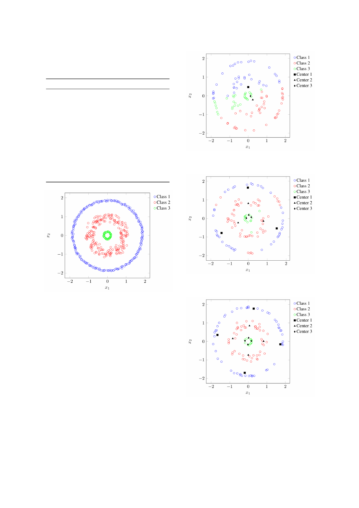
Table 5: Execution of cGA with simple split and using split

into three partitions (train, validation, and test partitions)

with cross-validation (CV) on the validation partition. 20

runs were executed.

Dataset Simple split Split with CV

Balance 12.02 15.77

Credit 13.34 12.62

Dermatology 4.95 5.60

Diabetes 21.61 21.41

E.Coli 14.32 13.09

Glass 37.36 33.68

Heart 18.60 21.93

Horse colic 33.91 32.88

Iris 1.62 1.35

Thyroid 3.49 3.58

WDBCancer 4.26 3.56

WDBCancer-Int 1.61 3.74

Wine 2.84 3.30

Figure 4: Distribution of samples into classes for the syn-

thetic ‘rings’ dataset.

served, the classiﬁcation error is signiﬁcantly reduced

with the addition of more clusters.

Although the addition of more clusters could solve

this speciﬁc clustering problem, it couldn’t improve

the classiﬁcation accuracy on the UCI datasets. This

indicate that the UCI datasets probably belong to the

third type mentioned in Section 4.6, where the exam-

ples of each class are mixed into confusion regions,

that are difﬁcult to tackle by a centroid based algo-

rithm.

6 CONCLUSIONS

In this work, a Cellular Genetic Algorithm has been

used to tackle the problem of classiﬁcation of pat-

terns into clusters. The algorithm was tested on 13

Figure 5: Classiﬁcation of the ‘rings’ dataset using one clus-

ter per class. The obtained classiﬁcation error is equal to

54.4643% (61 misclassiﬁed examples out of 112).

Figure 6: Classiﬁcation of the ‘rings’ dataset using three

clusters per class. The obtained classiﬁcation error is equal

to 11.6071% (13 misclassiﬁed examples out of 112).

Figure 7: Classiﬁcation of the ‘rings’ dataset using four

clusters per class. The obtained classiﬁcation error is equal

to 0%.

ECTA 2015 - 7th International Conference on Evolutionary Computation Theory and Applications

372

diverse benchmarks and compared with nine classiﬁ-

cation techniques and three metaheuristics.

Experiments show that the cGA is competitive

with the chosen special purpose classiﬁcation tech-

niques and also with the general purpose metaheuris-

tics, attaining the best result on one problem instance.

The cGA was ranked in ﬁfth place.

Regarding future developments, two points were

considered. The ﬁrst is test other crossover and mu-

tation operators, and verify if the hybridization of the

cGA with local search metaheuristics is able to im-

prove the basic cGA. The second point aims at per-

forming a more rigorous study of the population grid

layout, size, and neighbours used.

ACKNOWLEDGEMENTS

This work was partially supported by national funds

through Fundac¸

ao para a Ci

encia e a Tecnologia

(FCT) under project [UID/EEA/50009/2013], and by

the PROTEC Program funds under the research grant

[SFRH/PROTEC/67953/2010].

REFERENCES

Alba, E. and Dorronsoro, B. (2008). Cellular Genetic Algo-

rithms. Springer Publishing Company, Incorporated,

1st edition.

Borgelt, C. (2006). Prototype-based classiﬁcation and clus-

tering. PhD thesis, Otto-von-Guericke-Universit

Magdeburg, Universit

atsbibliothek.

Cahon, S., Melab, N., and Talbi, E.-G. (2004). Par-

adiseo: A framework for the reusable design of paral-

lel and distributed metaheuristics. Journal of Heuris-

tics, 10(3):357–380.

Duda, R. O., Hart, P. E., and Stork, D. G. (2000). Pattern

Classiﬁcation (2Nd Edition). Wiley-Interscience.

Falco, I. D., Cioppa, A. D., and Tarantino, E. (2007). Facing

classiﬁcation problems with particle swarm optimiza-

tion. Appl. Soft Comput., 7(3):652–658.

Falkenauer, E. (1998). Genetic Algorithms and Grouping

Problems. John Wiley & Sons, Inc., New York, NY,

USA.

Garc

ıa, S. and Herrera, F. (2008). An extension on “sta-

tistical comparisons of classiﬁers over multiple data

sets” for all pairwise comparisons. Journal of Ma-

chine Learning Research, 9:2677–2694.

Jain, A. K. (2010). Data clustering: 50 years beyond k-

means. Pattern Recognition Letters, 31(8):651 – 666.

Award winning papers from the 19th International

Conference on Pattern Recognition (ICPR)19th Inter-

national Conference in Pattern Recognition (ICPR).

Jain, A. K., Murty, M. N., and Flynn, P. J. (1999). Data

clustering: A review. ACM Comput. Surv., 31(3):264–

323.

Karaboga, D. and Ozturk, C. (2011). A novel clustering

approach: Artiﬁcial bee colony (abc) algorithm. Appl.

Soft Comput., 11(1):652–657.

Lichman, M. (2013). UCI machine learning repository.

University of California, Irvine, School of Informa-

tion and Computer Sciences.

Lourenc¸o, A., Bul

o, S. R., Rebagliati, N., Fred, A. L. N.,

Figueiredo, M. A. T., and Pelillo, M. (2015). Proba-

bilistic consensus clustering using evidence accumu-

lation. Machine Learning, 98(1-2):331–357.

Marinakis, Y., Marinaki, M., Doumpos, M., Matsatsinis, N.,

and Zopounidis, C. (2008). A hybrid stochastic genet-

icgrasp algorithm for clustering analysis. Operational

Research, 8(1):33–46.

Maulik, U., Bandyopadhyay, S., and B, S. (2000). Genetic

algorithm-based clustering technique. Pattern Recog-

nition, 33:1455–1465.

Mirkin, B. (1996). Mathematical Classiﬁcation and Clus-

tering. Kluwer Academic Publishers, Dordrecht, The

Netherlands.

Ni, J., Li, L., Qiao, F., and Wu, Q. (2013). A novel

memetic algorithm and its application to data cluster-

ing. Memetic Computing, 5(1):65–78.

Niknam, T. and Amiri, B. (2010). An efﬁcient hybrid ap-

proach based on pso, aco and k-means for cluster anal-

ysis. Appl. Soft Comput., 10(1):183–197.

Selim, S. Z. and Ismail, M. A. (1984). K-means-type algo-

rithms: A generalized convergence theorem and char-

acterization of local optimality. IEEE Trans. Pattern

Anal. Mach. Intell., 6(1):81–87.

Senthilnath, J., Omkar, S., and Mani, V. (2011). Clustering

using ﬁreﬂy algorithm: Performance study. Swarm

and Evolutionary Computation, 1(3):164 – 171.

Zhao, J., Lei, X., Wu, Z., and Tan, Y. (2014). Clustering

using improved cuckoo search algorithm. In Tan, Y.,

Shi, Y., and Coello, C., editors, Advances in Swarm

Intelligence, volume 8794 of Lecture Notes in Com-

puter Science, pages 479–488. Springer International

Publishing.

Clustering using Cellular Genetic Algorithms

373