Measuring Temporal Parameters of Gait with Foot Mounted IMUs in
Steady State Running
G. P. Bailey and R. K. Harle
Computer Laboratory, University of Cambridge, William Gates Building, 15 JJ Thomson Avenue, Cambridge, U.K.
Keywords:
Running, Gait, Temporal Gait Parameters, Foot Kinematics, Continuous Sensing, Toe-off, Heel-strike,
Cadence, Contact-time.
Abstract:
The continuous sensing of running biomechanics provides an opportunity to monitor changes in sporting tech-
nique for performance or injury prevention. Inertial sensors are now small enough to integrate into footwear,
providing a potential platform for continuous monitoring that does not require additional components to be
worn by the athlete and that can be used to assess foot kinematics during running as well as temporal parame-
ters. While temporal parameters of gait are already widely used, they may be combined with the measurement
of foot kinematics assessed using a wearable — Inertial Measurement Unit (IMU) based — foot mounted Iner-
tial Navigation System (INS). Assessment of foot pose at times of foot-ground interaction (such as heel-strike
and toe-off) is likely to require excellent accuracy in the face of changing technique and speed. We present and
evaluate a threshold free algorithm for assessing temporal gait parameters using a foot mounted IMU. We also
investigate the impact of errors in temporal gait parameters on the measurement of foot kinematics at these
time points. We find that our algorithm has good accuracy, for example we find a mean error 0.47 ± 3.84ms
for toe-off estimation at a running velocity of 3.4ms
−1
. We also find that the magnitude of this error has
little affect on some spatial parameter measurements, such as frontal plane foot angle (at a running speed
of 2.3ms
−1
, mean error at toe-off was 0.93 ± 2.07
◦
). However, for others the error in temporal parameters
produces larger changes, for example sagital plane foot angle (at a running speed of 2.3ms
−1
, mean error at
toe-off was 4.11
◦
± 3.70).
1 INTRODUCTION
Biomechanical assessment of movement is a compli-
cated but valuable component of todays elite sports
training. Assessment of running gait is particularly
important and is usually performed within a labo-
ratory setting. These assessments are often charac-
terised by expensive equipment, manual analysis and
subjective metrics. Furthermore the restricted space
of a laboratory necessitates evaluation either using a
small number of steps or, more often, a treadmill. In
neither case is the athlete free to move naturally and
there is little guarantee that the gait exhibited is that
found in the true sporting arena.
In order to address these issues and to bring
such biomechanical assessment to a wider audience,
low-cost inertial sensors are being embedded within
consumer products, allowing athletes to be assessed
in their natural setting and, additionally, more fre-
quently. Such in-field constant-assessment brings
with it additional benefits, including tracking the
progress of injury rehabilitation and enabling longi-
tudinal sports science and biomechanical studies
Foot-mounted sensors are popular since
lightweight sensors can be embedded within
shoes in a convenient, unobtrusive way. They may be
able to capture rich data, and have already attracted
commercial interest (e.g. the Nike+ shoe). In the
future, such sensors may be able to track relevant
performance metrics or detect poor or compensatory
patterns of gait.
Temporal parameters of gait are of particular inter-
est when measuring gait. These parameters include
the time of heel-strike and toe-off which in turn can
be used to assess other temporal parameters, such as
flight time, contact time, and cadence, all of which are
of interest to athletic coaches and biomechanists.
Temporal parameters of gait give important in-
formation regarding the gait cycle, for example con-
tact time (derived from the difference in time be-
tween heel-strike and toe-off events) is of use to sprint
coaches, where there is a relationship between contact
time and speed. Contact time has also been identified
as a useful measure of technique during a survey of
24
Bailey, G. and Harle, R..
Measuring Temporal Parameters of Gait with Foot Mounted IMUs in Steady State Running.
In Proceedings of the 3rd International Congress on Sport Sciences Research and Technology Support (icSPORTS 2015), pages 24-33
ISBN: 978-989-758-159-5
Copyright
c
2015 by SCITEPRESS – Science and Technology Publications, Lda. All rights reserved
athlete and coaches perceptions of technology needs
(Fleming et al., 2010) and has been suggested as a
method of assessing running skill level (Strohrmann
et al., 2012). Cadence may also be derived from tem-
poral parameters and is a useful clinical measurement
(Dugan and Bhat, 2005). It has been suggested that
reduction in stride length may reduce the probability
of stress fractures (Edwards et al., 2009), cadence is,
therefore, an important metric for coaches and ath-
letes since the only way to reduce stride length —
without a change in running velocity — is to increase
cadence. Cadence measurement may also be useful
for the coach or athlete trying to optimise cadence for
performance purposes.
Previous work has enabled the trajectory of the
foot to be assessed using foot worn sensors in both
running (Bailey and Harle, 2014) and walking (Mar-
iani et al., 2010). Foot trajectory may become even
more useful when combined with temporal parameter
measurement. The foot trajectory is a rich source of
information and it may be helpful to interpret it with
the help of temporal gait parameters. The foot makes
it’s contribution to locomotion while in contact with
the floor, this means it is important to know the cir-
cumstances in which the foot first made contact with
the ground, and further, the circumstances with which
it terminated contact with the floor.
Providing both temporal parameters and spatial
parameters of gait from data obtained from a shoe
mounted Inertial Measurement Unit (IMU) is desir-
able and since spatial parameters have been previ-
ously investigated (Bailey and Harle, 2014), assess-
ment of temporal parameters using a foot mounted
IMU is an important next step. The purpose of this
study is to provide an algorithm to estimate tempo-
ral parameters of gait using a foot mounted IMU. The
affects of the accuracy of temporal parameters on the
estimation of spatial parameters at heel-strike and toe-
off will also be investigated.
We address the following research questions:
• Is it possible to use a foot mounted IMU to mea-
sure temporal parameters of running gait?
Previous studies have used thresholds with ac-
celerometer data to assess temporal parameters or
running gait using a foot mounted IMU. While at-
tempting to use these methods to estimate toe-off
we have found them to be inaccurate and unreli-
able in the face of differing pace. Is it possible to
come up with an algorithm that doesn’t use thresh-
olds to assess temporal parameters of gait and how
accurate is it?
• How does the accuracy of heel-strike and toe-off
estimation affect the measurement of spatial pa-
rameters at these time points?
Previous work has used the strapdown inertial
navigation algorithm together with IMUs to re-
cover the trajectory of the foot during each gait
cycle in steady state running. Heel-strike and toe-
off time could be used in combination with the
trajectory of the foot to assess the pose of the foot
at these time points. What affect does the error in
temporal parameter estimation have on the accu-
racy of spatial measurements of gait at points in
time where the foot interacts with the ground.
2 BACKGROUND
Measurement of temporal parameters of gait using
wearable sensors for in situ monitoring has been stud-
ied in the recent past, however many of the studies
available have concentrated on walking gait or inves-
tigate temporal parameters with sensors attached to
areas of the body that are not the foot and — as as
previously stated — we believe that placing sensors
within the shoe is beneficial in terms of ease and fre-
quency of use. While there has been limited assess-
ment of temporal parameters in running using foot
mounted inertial sensors, many other studies have in-
vestigated temporal gait parameters either in walking
or in running using different sensor placements. Fur-
ther, different sensor systems have also been used,
such as pressure sensors. This section will describe
directly related previous work.
A previous work (Strohrmann et al., 2011) in-
vestigated the assessment of normalised foot contact
time using wearable sensors. To do so the time of
heel-strike and toe-off were estimated using a foot
mounted IMU. Placement of the sensor was on the in-
step of the shoe. Toe-off was detected when the accel-
eration magnitude exceeded a threshold of 2g follow-
ing a period where the magnitude of the acceleration
was below a particular threshold subsequent to the
detected foot strike. No formal evaluation was pre-
sented for the accuracy of the recovered toe-off and
foot-strike times, but in our experience this algorithm
is inaccurate and differing running pace produced sig-
nificantly different results.
Shank mounted gyroscopes have also been used
to assess contact times in running and walking (Mc-
Grath et al., 2012) where a gyroscope based algorithm
(Greene et al., 2010) was used to to determine heel-
strike and toe-off times. This was evaluated using
optical motion capture data with two different algo-
rithms (Zeni et al., 2008; Hreljac and Marshall, 2000)
applied, these algorithms present a limitation to this
study as they have been found to be inaccurate in run-
ning (Maiwald et al., 2009). The results showed poor
Measuring Temporal Parameters of Gait with Foot Mounted IMUs in Steady State Running
25
to moderate agreement for stance and swing times but
performed better for stride times.
While not based on inertial sensors, a number of
studies have used pressure sensors embedded within
shoes to assess temporal gait parameters. For exam-
ple, pressure sensors embedded within sprinters shoes
have been used to provide contact times (Harle et al.,
2011). While the system achieved results with a sim-
ilar accuracy to force plate data, pressure sensors can
be prone to break due to the wiring required and the
forces placed upon those wires (and to the sensors
themselves) during vigorous motion. For that reason,
we have chosen to target the use of IMUs instead of
pressure sensors due to the aims of enabling in situ
monitoring, potentially over a long period of time.
By using an IMU based approach we avoid overcom-
ing the problems with reliability of pressure sensors
and make the system viable for lay users and poten-
tial manufacturers alike.
2.1 Current Methods of Assessing
Temporal Parameters
Current methods of assessing temporal parameters are
commonly lab based. The ‘gold standard’ method
of temporal parameter assessment is the use of force
plates. Force plates provide a force/time series, in or-
der to derive temporal parameters a threshold is ap-
plied to the vertical component of the measured force
— this is called the Ground Reaction Force (GRF)
— to detect the increase in force applied to the plate
that corresponds to the contact phase of gait. This
threshold is typically set so that it is large enough
to be above the noise floor of the sensor and small
enough that there is minimal error in the timing, in
particular 10N is the typical threshold value (Hreljac
and Marshall, 2000; O’Connor et al., 2007; Maiwald
et al., 2009). The use of force plates for temporal gait
analysis methods has limitations however, and these
depend on how the force-plate is used. There are two
different scenarios in which the force plate is used,
the first is embedded into the floor of the laboratory
or running track and the second is embedded within a
treadmill.
When embedded into the floor or a running track
the area covered by a single force plate is limited to a
small area, typically only big enough to assess a sin-
gle step at a time. This means that the subject be-
ing assessed may modify their gait to hit the plate —
through adaptations of step length (Abendroth-Smith,
1996) and by extension either contact time or cadence
— or miss the area altogether. This means that col-
lecting data on a large number of steps is a laborious
task as many trials have to be discarded if the subject
modifies their gait or misses the plate and the discard-
ing of steps is subject to human judgement and may
be prone to error or bias. Furthermore, there may be
some instances where the sequence of steps leading
up to a particular manoeuvre, such as cutting, is of
importance. This can be very difficult to assess with
force plates and so video may be used introducing a
laborious and subjective digitisation task. Multiple
force plates may be embedded in the track/running
surface but the subject being assessed may not hit
each one, and the extra instrumentation is a large and
unwanted additional cost.
These limitations can to some extent be mitigated
by using a treadmill with an embedded force plate,
this is the other typical usage scenario. However, this
introduces new compromises. Firstly, gait exhibited
on a treadmill may be different to that of walking
or running over ground, particularly if the subject is
unfamiliar with using a treadmill. Secondly, the me-
chanical nature of the treadmill introduces noise to
the force-plate data meaning that the threshold used to
find contact times must be increased accordingly, pre-
vious studies have used a threshold of 20N (for exam-
ple (Zeni et al., 2008)). This affects accuracy and con-
sistency with studies based on overground running,
the higher threshold may lead to later estimates of
heel-strike and earlier estimates of toe-off when com-
pared to overground force-plate data. Also, more am-
bitious studies looking at at a series of contact times
prior to a manoeuvre (such as cutting) are impossible
on a treadmill. Finally, they are expensive and rela-
tively uncommon.
The limitations of the above two scenarios suggest
a need to be able to assess temporal parameters in-situ
but with the ability to assess each step in sequence.
3 SENSOR PLATFORM AND
DATA CAPTURE
3.1 Inertial Sensors
Capture of inertial sensor data was facilitated using
the ION (Imperceptible On-body Node) sensor plat-
form (Harle et al., 2011) with the addition of an
IMU providing a three-axis ±16g accelerometer and
±2000
◦
s
−1
gyroscope (MPU-6000, InvenSense Inc.)
and containing an internal 16 bit Analog-Digital Con-
verter (ADC). The sensor platform is lightweight,
weighing approximately 15 grams in total, including
battery.
All IMU signals were sampled at 1kHz and logged
to on-board flash memory. In all experiments the ION
icSPORTS 2015 - International Congress on Sport Sciences Research and Technology Support
26
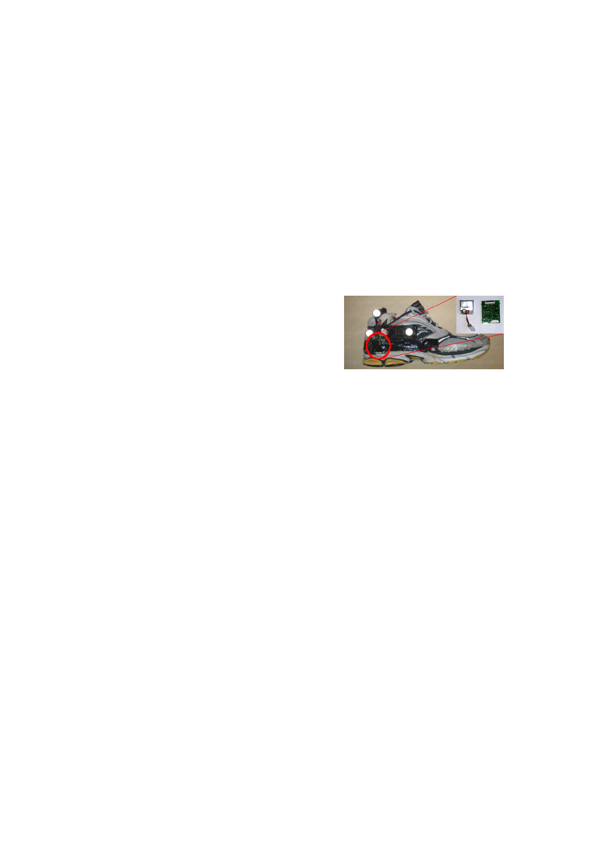
sensor was placed on the lateral side of the shoe in
line with the ankle, as seen in Figure 1. The sensor
was firmly taped to the outside of the shoe to simu-
late the scenario where it was built into the shoe, per-
haps embedded in the sole in a similar manner to the
Nike+ shoe. Since the algorithm presented in this pa-
per is intended for use along side an Inertial Naviga-
tion System (INS) the placement on the side of the
ankle is informed from an investigation into the valid-
ity of the zero-velocity assumption (Foxlin, 2005). It
has been shown that the sensor position we have used
is among the best suited to using this assumption dur-
ing a study of foot mounted inertial navigation tech-
niques, including an investigation of different mount-
ing locations on the foot (Peruzzi et al., 2011).
3.2 Ground Truth
Ground truth is important for assessing the ability
of any system to assess temporal parameters of gait.
However, the gold standard ground truth of a force
plate was unavailable due to a lack of equipment. Ac-
cess to an optical motion capture system (Vicon) was
available however. Previous studies have attempted to
validate algorithms based on kinematic data from mo-
tion capture to facilitate temporal parameter estima-
tion, these studies have typically focused on walking
gait. In order to validate kinematic data based tempo-
ral parameter estimation in running a previous study
(Maiwald et al., 2009) selected several potential al-
gorithms to evaluate in a running context including
their own ‘Foot Contact Algorithm’ (FCA). The eval-
uation of kinematic data based algorithms for tempo-
ral parameters proceeded with comparison to ground
reaction force data. They found that previously used
algorithms had problems with accuracy but their FCA
algorithm was reported to be accurate in both mea-
surement of heel-strike and toe-off with a similar ac-
curacy and precision to the ground reaction force de-
rived measurement. Therefore, we implemented this
algorithm to use as ground truth for evaluating our
IMU algorithm.
Kinematic data was captured using an optical mo-
tion capture system (Vicon Motion Systems, UK)
sampling at 240Hz. A treadmill was used in order to
capture many steps in a limited motion capture area.
The treadmill was set up without any inclination as
measured with a spirit level. The ION sensor was
attached to a custom jig containing 3 retro-reflective
markers (Fig. 1) for the motion capture system, this
setup was previously used to evaluate trajectory re-
covery using a foot-mounted IMU (Bailey and Harle,
2014). The jig in this instance facilitates estimation
of the pose of the foot, and the data is used in order to
assess the affect of errors in temporal parameters on
the estimation of associated spatial parameters. We
use the motion capture data when measuring the af-
fect of temporal parameter error on spatial parameter
determination to isolate the error cause by the tempo-
ral parameters from the potential errors incurred using
an INS solution.
The jig adds an additional 30 grams of weight to
the system (45 grams total, including ION) but re-
mains comfortable for test runs. The jig was laser cut
and the MPU-6000 and retro-reflective markers were
aligned with laser-etched outlines to ensure alignment
between the jig and the inertial sensor axes. An addi-
tional marker was placed on the toe to facilitate using
the FCA algorithm. The posterior marker on the jig
was used as the heel marker for the FCA algorithm.
Figure 1: Shoe with IMU and Jig for facilitating ground
truth capture using the Vicon Motion capture system.
3.3 Data Collection
In order to evaluate the temporal parameter estima-
tion algorithm presented in this paper data were col-
lected from 5 participants. Each participant ran for
90 seconds at 4 different speeds. After detection of
the running period, 90 steps were extracted for each
participant at each speed to ensure the same number
of steps were used for each participant. After select-
ing these 90 steps the heel-strike and toe-off detection
was performed for each step. This produced a total of
1800 steps for analysis.
4 TEMPORAL PARAMETER
ALGORITHM
The algorithm proposed in this section takes a divide
and conquer approach to finding temporal parameters.
Data files are first segmented to find periods of run-
ning (run detection), followed by identifying regions
that contain a single step from heel-strike to toe-off
(step segmentation). Once regions containing heel-
strike and toe-off events from a single step are iden-
tified, consistent features of the step are used to seg-
ment the signal further to get more accurate temporal
parameter estimations.
Measuring Temporal Parameters of Gait with Foot Mounted IMUs in Steady State Running
27
4.1 Running Detection and Step
Segmentation
This section will describe the process of run detection
and step segmentation before returning to the tempo-
ral parameter estimation later.
4.1.1 Normalised Auto-correlation based Step
Counting
A modified version of the Normalised Auto-
correlation based Step Counting algorithm (NASC
(Rai et al., 2012)) is used to first detect periods of
running and then to roughly segment the signal into
individual steps for further inspection to find tempo-
ral parameters.
The NASC algorithm exploits the periodicity of
gait in order to detect periods of walking. The al-
gorithm uses auto-correlation of an inertial signal.
Given that inertial signals measured during gait are
periodic the auto-correlation value should be at it’s
largest at the correct periodicity of the gait cycle. The
NASC algorithm was developed to work with inertial
sensors placed in any location on the body to detect
walking via detecting periodic motion. In this case,
the location of the sensor is known and the mode of
gait is running rather than walking. This means that
the algorithm is modified accordingly to take advan-
tage of this knowledge.
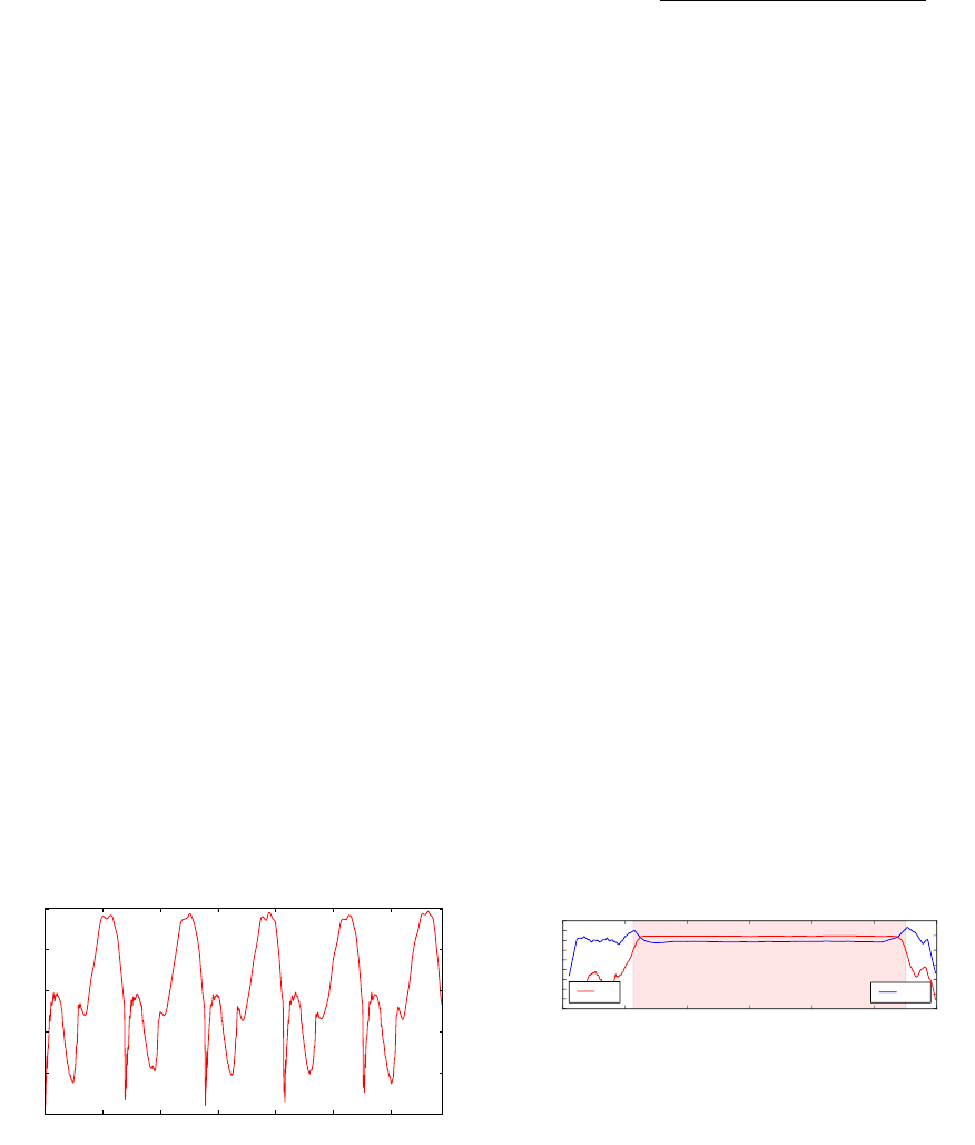
The original algorithm uses the acceleration sig-
nal for walk detection. For this work, sagital plane
angular rate (g
z
) is used since there is lower noise and
higher step to step repeatability with this signal for
our particular application using a foot-mounted IMU.
This can be seen in Figure 2.
0 500 1000 1500 2000 2500 3000
Time (ms)
−15
−10
−5
0
5
10
g
ion
z
(rad/s)
Figure 2: Example showing five steps of sagital plane angu-
lar rate (g
ion
z
).
Given a signal — in this case g
ion
z
(n) — the NASC
algorithm computes the normalised auto-correlation χ
for lag τ at the m
th
sample as described by the follow-
ing two equations that have been split for readability.
χ(m, τ) =
∑
k=τ−1
k=0
[α(m,τ,k)α(m+τ,τ,k)]
τσ(m,τ)σ(m+τ,τ)
(1)
α(i, τ, k) = g
ion
z
(i + k) − µ(i, τ) (2)
In Equations 1 and 2, µ(k, τ) and σ(k, τ) are the
mean and standard deviation of the sequence of sam-
ples < g
ion
z
(k), g
ion
z
(k + 1), ..., g
ion
z
(k + τ − 1) >.
When the subject wearing the sensor is running
(or walking) and τ is exactly equal to the period of the
acceleration pattern, the normalised auto-correlation
will be close to one. However, τ is unknown and
so NASC tries values of τ between selected values of
τ
min
and τ
max
to find the value of τ for which χ(m, τ)
becomes maximum (τ
opt
). This is described by the
following equation.
ψ(m) = max
τ=τ
max
τ=τ
min
(χ(m, τ)) (3)
The implementation presented in (Rai et al., 2012)
used a search window (τ
min
,τ
max
) of (0.8s,2s) for
walking, this is based on the typical two step duration
of walking. However our scenario is treadmill run-
ning and so a search window of (0.6s, 0.9s) is used
based on the cadence of the runners tested during the
experiments in this paper.
The maximum normalised auto-correlation, ψ(m),
simultaneously provides two pieces of information
(Rai et al., 2012). Firstly, a high value (close to 1)
suggests that the person is running or walking since
it implies a high level of repeatability in the signal
in typical gait cadence ranges, this can be used for
run (or walk) detection,. Secondly, the corresponding
value of τ = τ
opt
gives the periodicity of the persons
gait. A moving average filter with a 5 second window
is used for both ψ(m) and τ
opt
signals and an example
of the resulting signals is given in Figure 3.
0 20000 40000 60000 80000 100000 120000
0
100
200
300
400
500
600
700
800
900
τ
opt
(ms)
τ
opt
0.0
0.2
0.4
0.6
0.8
1.0
ψ(m)
ψ
Figure 3: Graph showing τ
opt
and ψ(m) with 5s moving
average filter applied. Shaded area shows the period of de-
tected running.
4.1.2 Run Detection
Periods of running are detected in a similar manner
to (Rai et al., 2012). However, since the experi-
ments here are constrained to small data files where
we know that running forms the majority of the file, a
simpler algorithm is used that doesn’t take account of
previous states and only uses a threshold on the value
of ψ(m). A threshold value of 0.8 is used, any value
icSPORTS 2015 - International Congress on Sport Sciences Research and Technology Support
28
of ψ(m) above 0.8 is deemed to be a period of running
(Figure 3). This detection method would likely need
to take into account previous states as in (Rai et al.,
2012) were the file to consist of more free form mo-
tion with periods of running interspersed with other
activities. This was outside of the scope of the current
work.
4.1.3 Single Step Segmentation
The NASC algorithm was originally designed for step
counting (Rai et al., 2012), however, we are interested
in segmenting the steps rather than counting them and
therefore the algorithm was modified for this work in
order to segment steps. An additional requirement is
that it needs be robust to changes in speed and there-
fore should not rely on thresholds.
Setting thresholds is not desirable as they are not
robust to changes in running technique, running ve-
locity and other factors that affect the magnitude of
the peaks of the inertial measurements. This makes
robust algorithms that yield few false positives hard
to code. This also removes the need for constraints —
such as detection of improbable cadences — that are
required in order to detect missed peaks due to them
being lower than the threshold used.
The NASC algorithm not only enables robust de-
tection of running steps, but the value of t
opt
(m) gives
an estimate of the time between heel-strike events,
this could otherwise be described as the gait period
(or the inverse of cadence). This information can be
used in order to segment steps based on some repeat-
able and easily detectable signal feature.
The segmentation proceeds by first looking for
one of the clear peaks in the g
ion
z
signal near to t
start
,
the start time of the detected period of running. In
order to avoid thresholds we look for the maximum
value of g
ion
z
in the first two seconds.
ts(1) = time(max
t=t
start
+2τ
opt
(t
start
))
t=t
start
(g
ion
z
(t))) (4)
Here, ts(1) is the time of the first step segment.
This may end up missing a single step at the start,
this is due to the size of the initial search window.
This window contains approximately two steps worth
of data either of which could contain the maximum
value so the first is not necessarily selected. This gives
a clear and simple to implement method of gaining a
single peak to identify as a start point for further seg-
mentation. The peak detected represents the start of
the first step segment. The time of subsequent seg-
ments are found using in a similar manner by looking
in a window defined by the periodicity of the run at
the last peak τ
opt
(ts(n)), where n is the segment num-
ber.
ts(n + 1) = time(max
t=ts(n)+
6τ
opt
(ts(n))
5
t=ts(n)+
τ
opt
(ts(n))
2
(g
ion
z
(t))) (5)
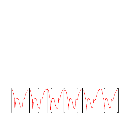
This results in rough segmentation from which the
temporal parameters can be further refined. Figure
4 shows an example of the results of segmentation.
Each segment (ts(n), ts(n + 1)) is guaranteed to con-
tain a heel-strike and toe-off event, this is because the
maximum sagital plane angular rate of the foot is dur-
ing the flight phase of gait. This makes identifying
these events a much simpler task that attempting to
identify correctly all heel-strike events given a period
of data containing multiple steps.
0 500 1000 1500 2000 2500 3000 3500 4000
Time (ms)
−15
−10
−5
0
5
10
g
ion
z
(rad/s)
Figure 4: Segmentation of g
ion
z
using NASC algorithm to
find successive peaks, vertical lines show start times of suc-
cessive segments (ts(n)).
4.2 Finding Heel-strike and Toe-off
Points
Now that the running file has been segmented into
sections each containing a single heel-strike and toe-
off event, the algorithm further splits the step into
easy to find pieces before attempting to find the more
subtle features associated with heel-strike and toe-off
events. The process for each event will be described
in the following sections.
4.2.1 Heel-strike
Heel-strike is found by looking for the large changes
in signal associated with heel-strike. We again use the
g
ion
z
signal for this task due to it having relatively little
noise compared with the accelerometer signal.
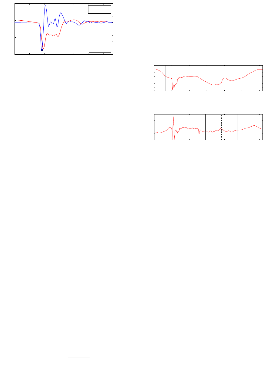
Large changes in a signal can be more easily de-
tected by assessing the first differential. Heel-strike
is assessed by inspecting the signal in a region de-
fined using the course segmentation defined in Sec-
tion 4.1.3, sagital plane angular rate for a subset of
a region (ts(n), ts(n + 1)) is shown in Figure 5. For
each coarse segment, the differential of the g
ion
z
signal
is calculated. Then the minimum value of the result-
ing signal is found, this is shown as the marked circle
in Figure 5 and defined in Equation 6.
t
ˆ
hs
(n) = time(min
t=ts(n)
t=ts(n+1)
(g
0ion
z
(t))) (6)
Here t
ˆ
hs
(n) is the first estimate of the time of heel
strike for step n, ts(n) is the time of the start of a
Measuring Temporal Parameters of Gait with Foot Mounted IMUs in Steady State Running
29
200 220 240 260 280 300 320
−20
−15
−10
−5
0
5
10
g
ion
z
(rad/s)
g
ion
z
−5
−4
−3
−2
−1
0
1
2
3
g0
ion
z
(rad/s
2
)
g0
ion
z
Figure 5: Heel-strike detection from sagital plane angular
rate.
coarse segment for step n and g0
ion
z
(t) is the differen-
tial of the g
ion
z
(t) signal. This detects a rough estimate
for the time of heel-strike which is then refined in the
following way.
The peak in the differential represents the max-
imum rate of change, but this is logically after the
heel-strike due to the deformity of the mid-sole of the
shoe on impact meaning that the true time of heel-
strike should be at the base of this peak. Therefore
this estimate is refined by seeking backwards in time
to find the base of the local minima. Therefore the al-
gorithm seeks backwards from t
ˆ
hs
(n) up to the point
where g0
ion
z
(t) is greater than -0.5, this point is then
taken to be the detected heel-strike event t
hs
(n). The
detected time of heel-strike is shown as the vertical
dashed line in Figure 5.
4.2.2 Toe-off
While heel-strike has associated large peaks in in-
ertial data that are easy to detect, the way the foot
peels away from the floor before toe-off means that
large signal changes don’t exist at toe-off using a heel
mounted IMU. The best algorithm found by us for
toe-off with a heel-mounted sensor depends on find-
ing a small local maxima, in the a
ion
y
(t) signal. The
a
ion
y
(t) channel is aligned with the shank during static
standing. As this local maxima is relatively small it
is hard to find a reliable algorithm to detect it without
further segmentation of the step. Further segmenta-
tion of the step allows easier detection of the relevant
local maxima.
The segmentation is done by finding the zero
crossing in the g
ion
z
(t) signal as shown by the verti-
cal lines in Figure 6a. Once the zero crossings are
found we look in a window defined using the follow-
ing formulae.
w
start
= c
0
+
(c
1
+ c
0
)
2
(7)
w
end
=
4(c
1
− w
start
)
5
+ w
start
(8)
Here, w
start
and w
end
are the times of the start
and end of the window respectively and c
0
and c
1
are
the first and second zero crossings. This window is
marked by the vertical lines in Figure 6b. This nar-
rows down the signal enough that we can now re-
liably find the minima in the a
ion
y
(t) signal between
w
start
and w
end
, this point corresponds to toe-off (Fig-
ure 6b).
0 100 200 300 400 500 600
Time (ms)
−20
−15
−10
−5
0
5
10
15
g
z
(rad/s)
(a) Further segmentation using zero crossings is demonstrated
by the vertical lines.
0 100 200 300 400 500 600
Time (ms)
−50
0
50
a
y
(ms
−2
)
(b) Toe-off detection. Solid vertical lines show w
start
and w
end
,
dashed vertical line shows detected toe-off.
Figure 6: Further segmentation in order to find toe-off.
This point is less well defined at slower speeds how-
ever and may impact upon the accuracy at slower
speeds, this is shown in the results of the evaluation.
4.3 Applicability
We have chosen the above algorithm after trying
many other potential algorithms. This algorithm has
the disadvantage that it is most likely dependant on
sensor position, particularly alignment, however the
alignment chosen for the the sensor and shoe should
be easy to replicate with the sensor built into the shoe
as it is positioned roughly perpendicular to the sur-
faces of the mid-sole. It should also be possible to
make small changes to the algorithm for differing
alignment such as swapped axes directions meaning
finding minimum points need to be substituted for
maximum points, for example. This should mean the
algorithm remains applicable to a sensor system built
into the shoe, but may not be sufficiently general for
an inertial system attached, for example, to the laces
of a standard shoe.
4.4 Evaluation
The errors in heel-strike and toe-off estimation us-
ing the inertial sensor based algorithm in this section
are presented in Table 1. The results show mixed ac-
curacy between different running speeds and are de-
icSPORTS 2015 - International Congress on Sport Sciences Research and Technology Support
30
pendant on the temporal parameter being assessed.
At lower speeds there is slightly lower accuracy and
higher variability in the toe-off metric, this is due to
the peak in a
ion
y
used to assess toe-off being wider and
not as sharp leading to less precise estimates at lower
speeds. The heel-strike assessment is not subject to
this problem due to the relatively large peaks associ-
ated with heel-strike.
Table 1: Mean and Standard Deviation of Errors estimating
temporal parameters in comparison to those derived from
the FCA algorithm. TO = Toe-Off, HS = Heel-Strike.
Speed Error TO (ms) Error HS (ms)
2.3ms
−1
12.63 ± 9.90 9.86 ± 6.99
2.7ms
−1
6.95 ± 7.74 9.91 ± 4.61
3.0ms
−1
2.48 ± 5.99 9.82 ± 3.98
3.4ms
−1
0.47 ± 3.84 9.89 ± 3.37
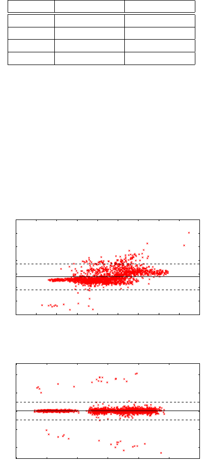
Contact times were derived from the results of
the inertial algorithm for comparison with previous
methods demonstrated earlier in this chapter. A small
bias of -4.37ms was found with limits of agreement
-23.50ms to 14.76ms. A Bland-Altman plot can be
seen in Figure 7. Cadence was also calculated and a
Bland-Altman plot of the results can be seen in Fig-
ure 8, there is a small bias of 0.002 steps per minute
and limits of agreement of 2.45 to -2.49 steps per
minute, however the figure demonstrates that occa-
sionally there are significant outliers.
200 220 240 260 280 300 320 340 360 380
Mean Contact Time (ms)
−60
−40
−20
0
20
40
60
80
Contact Time Difference (ms)
Figure 7: Bland-Altman plot of contact times derived from
a heel mounted IMU.
130 140 150 160 170 180 190
Mean Cadence (steps per minute)
−10
−5
0
5
10
Cadence difference (steps per minute)
Figure 8: Bland-Altman plot of cadence derived from a heel
mounted IMU.
5 AFFECT OF TEMPORAL
PARAMETER ESTIMATION
ERRORS ON SPATIAL
PARAMETER MEASUREMENT
An algorithm for determining heel-strike and toe-off
times using a heel mounted IMU has been presented
and evaluated. One of the reasons for developing such
an algorithm is to be able to evaluate spatial parame-
ters of gait using foot mounted INS methods (Bailey
and Harle, 2014). The temporal parameter estimation
described in the previous section is not perfect and has
some associated error. This section investigates how
that error affects the estimation of spatial parameters
of gait at heel-strike and toe-off events.
5.1 Evaluation Method
The FCA algorithm provided heel-strike and toe-off
times and the jig data were used to derive the angle
of the foot at these time points. The angle of the foot
is used as a potentially interesting spatial parameter
that might be evaluated at toe-off and heel-strike but
any other metric could potentially be calculated. At
heel-strike the angles of the foot in the sagital plane
(θ
s
(t)) and frontal plane θ
f
(t) were evaluated for each
step i from the Vicon data. These angles were also
evaluated at toe-off.
Further, the angle of the foot was recorded for
each step at multiple time points, calculated as offsets
from the output of the FCA algorithm. For example,
for step i, θ
s
(t) would be calculated for a sequence
of times t =< t
hs
(i)− 20, t
hs
(i)− 10, t
hs
(i)+ 0, t
hs
(i)+
10,t
hs
(i) + 20 > (times measured in milliseconds).
This series of measurements are designed to show the
progression of foot angle (an example of a spatial pa-
rameter) in the time period around the temporal event
of interest in order to assess accuracy requirements
for temporal parameters. Finally, foot orientation dif-
ferences are measured between time points measured
using the output of the ION based temporal parameter
estimation and FCA measured time points.
5.2 Results
The angles calculated from the Vicon data at various
time points are then turned into deltas from the angle
at t = t
hs
(i), for example θ
s
(t
hs
(i) − 20) − θ
s
(t
hs
(i)).
The results are shown in Table 2. The results show
that the error depends on the measurement being
taken, for example the error in the frontal plane at toe
off is relatively unchanged 20ms prior to and 20ms
after toe-off but the sagital plane angle varies greatly.
Measuring Temporal Parameters of Gait with Foot Mounted IMUs in Steady State Running
31
This indicates that the spatial parameter being mea-
sured may greatly affect the measurement accuracy
of temporal parameters required for accurate spatial
parameter measurement.
Table 2: Foot angle error at particular time offsets.
Measurement Error (ms)
θ
f
(t
f ca
hs
(i) − 20) − θ
f
(t
f ca
hs
(i)) 0.87 ± 1.43
θ
f
(t
f ca
hs
(i) − 10) − θ
f
(t
f ca
hs
(i)) 0.58 ± 1.07
θ
f
(t
f ca
hs
(i) + 10) − θ
f
(t
f ca
hs
(i)) 2.96 ± 2.15
θ
f
(t
f ca
hs
(i) + 20) − θ
f
(t
f ca
hs
(i)) 5.11 ± 2.95
θ
s
(t
f ca
hs
(i) − 20) − θ
s
(t
f ca
hs
(i)) −6.25 ± 1.91
θ
s
(t
f ca
hs
(i) − 10) − θ
s
(t
f ca
hs
(i)) −5.40 ± 1.38
θ
s
(t
f ca
hs
(i) + 10) − θ
s
(t
f ca
hs
(i)) 6.77 ± 1.36
θ
s
(t
f ca
hs
(i) + 20) − θ
s
(t
f ca
hs
(i)) 12.28 ± 2.22
θ
f
(t
f ca
to
(i) − 20) − θ
f
(t
f ca
to
(i)) 1.72 ± 1.67
θ
f
(t
f ca
to
(i) − 10) − θ
f
(t
f ca
to
(i)) 0.48 ± 1.06
θ
f
(t
f ca
to
(i) + 10) − θ
f
(t
f ca
to
(i)) 0.02 ± 1.37
θ
f
(t
f ca
to
(i) + 20) − θ
f
(t
f ca
to
(i)) 0.23 ± 2.93
θ
s
(t
f ca
to
(i) − 20) − θ
s
(t
f ca
to
(i))
7.81 ± 1.77
θ
s
(t
f ca
to
(i) − 10) − θ
s
(t
f ca
to
(i)) 3.72 ± 0.92
θ
s
(t
f ca
to
(i) + 10) − θ
s
(t
f ca
to
(i)) −2.78 ± 0.71
θ
s
(t
f ca
to
(i) + 20) − θ
s
(t
f ca
to
(i)) −5.04 ± 1.38
Table 3: Foot angle error between FCA and ION.
Measurement Speed Error (ms)
θ
s
(t
ion
hs
(i)) − θ
s
(t
f ca
hs
(i)) 2.3ms
−1
−4.56 ± 2.02
2.7ms
−1
−5.18 ± 1.68
3.0ms
−1
−5.79 ± 1.60
3.4ms
−1
−6.60 ± 2.04
θ
f
(t
ion
hs
(i)) − θ
f
(t
f ca
hs
(i)) 2.3ms
−1
0.33 ± 1.25
2.7ms
−1
0.46 ± 1.16
3.0ms
−1
0.71 ± 1.25
3.4ms
−1
0.71 ± 1.18
θ
s
(t
ion
to
(i)) − θ
s
(t
f ca
to
(i)) 2.3ms
−1
4.11 ± 3.70
2.7ms
−1
2.51 ± 2.82
3.0ms
−1
1.06 ± 2.51
3.4ms
−1
0.22 ± 1.64
θ
f
(t
ion
to
(i)) − θ
f
(t
f ca
to
(i)) 2.3ms
−1
0.93 ± 2.07
2.7ms
−1
0.08 ± 1.12
3.0ms
−1
0.14 ± 0.97
3.4ms
−1
0.14 ± 0.52
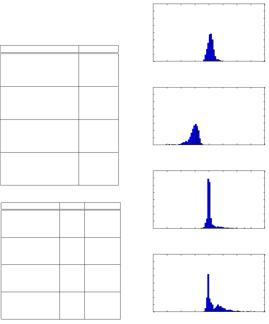
Figure 9 shows the distribution of errors for foot
angles at both toe-off and heel-strike and includes re-
sults for all speeds. Errors at heel-strike show similar
results to those at toe-off with the sagital plane be-
ing most affected. The mean error in frontal plane
angle at heel-strike between heel-strike measured by
FCA vs. ION was 0.56 ± 1.22 degrees. By contrast
the mean sagital plane error was −5.56 ± 2.01 de-
−20 −15 −10 −5 0 5 10 15 20
∆Angle(Degrees)
0
100
200
300
400
500
600
700
800
Frequency
(a) θ
f
(t
ion
hs
(i)) − θ
f
(t
f ca
hs
(i)).
−20 −15 −10 −5 0 5 10 15 20
∆Angle(Degrees)
0
100
200
300
400
500
600
700
800
Frequency
(b) θ
s
(t
ion
hs
(i)) − θ
s
(t
f ca
hs
(i)).
−20 −15 −10 −5 0 5 10 15 20
∆Angle(Degrees)
0
100
200
300
400
500
600
700
800
Frequency
(c) θ
f
(t
ion
to
(i)) − θ
f
(t
f ca
to
(i)).
−20 −15 −10 −5 0 5 10 15 20
∆Angle(Degrees)
0
100
200
300
400
500
600
700
800
Frequency
(d) θ
s
(t
ion
to
(i)) − θ
s
(t
f ca
to
(i)).
Figure 9: Difference in foot angle at temporal events mea-
sured by the ION and FCA algorithms.
grees. Again, this shows the magnitude of errors in
spatial parameters that are affected by a difference in
measured temporal parameters from reality is depen-
dant on the spatial parameter being measured. Re-
icSPORTS 2015 - International Congress on Sport Sciences Research and Technology Support
32
sults may also be dependant on individual technique,
Figure 9d shows a small secondary peak at 4 degrees
while the main peak is centred on 0 degrees. This may
mean that measurement error depends on an individ-
ual athletes technique as well as the measurement be-
ing evaluated.
Table 3 shows the angular errors obtained for the
time difference between the ION temporal parameters
algorithm and the FCA algorithm, broken down by
speed. The table shows that the slowest speeds have
the largest error for foot angle in the sagital plane but
the frontal plane is again relatively unaffected.
6 CONCLUSIONS
A method of reliably finding temporal parameters of
gait from a foot mounted IMU has been presented and
evaluated. The method presented is free of thresh-
olds that may be unreliable in the face of changing
technique and running pace. However, it is likely that
the algorithm will only work with the sensor position
used within this paper. The algorithm was designed
with a view to the sensors being built into the mid-sole
of the shoe so we view this as a minor limitation. The
algorithm has usable accuracy for temporal parameter
estimation but its accuracy for toe-off is somewhat de-
pendant on running velocity. The impact of the mag-
nitude of this error on the estimation of spatial metrics
was also investigated and shows that some metrics are
likely to be more affected than others. We find that
for some metrics there are minimal errors in spatial
parameters measured at time points derived from the
foot IMU data. Further work should seek to evaluate
the temporal parameter algorithm to check for accu-
racy and robustness in outdoor over ground running
to enable practical training and biomechanical assess-
ment tools.
REFERENCES
Abendroth-Smith, J. (1996). Stride Adjustments during a
Running Approach toward a Force Plate. Research
Quarterly for Exercise and Sport, 67(1):97–101.
Bailey, G. and Harle, R. (2014). Assessment of Foot Kine-
matics During Steady State Running Using a Foot-
mounted IMU. Procedia Engineering, 72:32–37.
Dugan, S. A. and Bhat, K. P. (2005). Biomechanics and
analysis of running gait.
Edwards, W. B., Taylor, D., Rudolphi, T. J., Gillette, J. C.,
and Derrick, T. R. (2009). Effects of stride length
and running mileage on a probabilistic stress fracture
model. Medicine and Science in Sports and Exercise,
41:2177–2184.
Fleming, P., Young, C., Dixon, S., and Carr
´
e, M. (2010).
Athlete and coach perceptions of technology needs for
evaluating running performance. Sports Engineering,
13(1):1–18.
Foxlin, E. (2005). Pedestrian tracking with shoe-mounted
inertial sensors. IEEE Computer Graphics and Appli-
cations, 25(6):38–46.
Greene, B. R., McGrath, D., O’Neill, R., O’Donovan, K. J.,
Burns, A., and Caulfield, B. (2010). An adaptive
gyroscope-based algorithm for temporal gait analysis.
Medical and Biological Engineering and Computing,
48:1251–1260.
Harle, R., Taherian, S., Pias, M., Coulouris, G., Hopper, A.,
Cameron, J., Lasenby, J., Kuntze, G., Bezodis, I., Ir-
win, G., and Kerwin, D. G. (2011). Towards real-time
profiling of sprints using wearable pressure sensors.
Computer Communications.
Hreljac, A. and Marshall, R. N. (2000). Algorithms to deter-
mine event timing during normal walking using kine-
matic data. Journal of Biomechanics, 33:783–786.
Maiwald, C., Sterzing, T., Mayer, T., and Milani, T. (2009).
Detecting foot-to-ground contact from kinematic data
in running. Footwear Science, 1(2):111–118.
Mariani, B., Hoskovec, C., Rochat, S., B
¨
ula, C., Penders, J.,
and Aminian, K. (2010). 3D gait assessment in young
and elderly subjects using foot-worn inertial sensors.
Journal of Biomechanics, 43:2999–3006.
McGrath, D., Greene, B. R., ODonovan, K. J., and
Caulfield, B. (2012). Gyroscope-based assessment of
temporal gait parameters during treadmill walking and
running. Sports Engineering, 15(4):207–213.
O’Connor, C. M., Thorpe, S. K., O’Malley, M. J., and
Vaughan, C. L. (2007). Automatic detection of
gait events using kinematic data. Gait and Posture,
25:469–474.
Peruzzi, A., Della Croce, U., and Cereatti, A. (2011). Es-
timation of stride length in level walking using an in-
ertial measurement unit attached to the foot: A vali-
dation of the zero velocity assumption during stance.
Journal of Biomechanics, 44:1991–1994.
Rai, A., Chintalapudi, K. K., Padmanabhan, V. N., and Sen,
R. (2012). Zee: Zero-Effort Crowdsourcing for Indoor
Localization. In Proceedings of the 18th annual in-
ternational conference on Mobile computing and net-
working - Mobicom ’12, page 293.
Strohrmann, C., Harms, H., Tr
¨
oster, G., Hensler, S., and
M
¨
uller, R. (2011). Out of the lab and into the woods:
kinematic analysis in running using wearable sensors.
In Proceedings of the 13th international conference on
Ubiquitous computing, pages 119–122. ACM.
Strohrmann, C., Rossi, M., Arnrich, B., and Troster, G.
(2012). A Data-Driven Approach to Kinematic Anal-
ysis in Running Using Wearable Technology. 2012
Ninth International Conference on Wearable and Im-
plantable Body Sensor Networks, pages 118–123.
Zeni, J. A., Richards, J. G., and Higginson, J. S. (2008).
Two simple methods for determining gait events dur-
ing treadmill and overground walking using kinematic
data. Gait and Posture, 27:710–714.
Measuring Temporal Parameters of Gait with Foot Mounted IMUs in Steady State Running
33
