raxDAWN: Circumventing Overﬁtting of the Adaptive xDAWN

Mario Michael Krell

, Hendrik W

ohrle

and Anett Seeland

Robotics Research Group, University of Bremen, Robert-Hooke-Str. 1, Bremen, Germany

Robotics Innovation Center, German Research Center for Artiﬁcial Intelligence GmbH, Bremen, Germany

Keywords:

xDAWN, Spatial Filtering, Online Learning, Electroencephalogram, Event-Related Potential, Brain-Computer

Interface.

Abstract:

The xDAWN algorithm is a well-established spatial ﬁlter which was developed to enhance the signal quality

of brain-computer interfaces for the detection of event-related potentials. Recently, an adaptive version has

been introduced. Here, we present an improved version that incorporates regularization to reduce the inﬂuence

of noise and avoid overﬁtting. We show that regularization improves the performance signiﬁcantly for up to

4%, when little data is available as it is the case when the brain-computer interface should be used without or

with a very short prior calibration session.

1 INTRODUCTION

In brain-computer interfaces (Blankertz et al., 2011;

Zander and Kothe, 2011; van Erp et al., 2012;

Kirchner et al., 2013, BCIs), event-related potentials

(ERPs) in the electroencephalogram (EEG) are quite

often used to deduce informations from the human’s

internal brain state and translate the internal state to

informations that are usable by other systems. Exam-

ples are P300 and error related potentials (Krusien-

ski et al., 2006; Buttﬁeld et al., 2006). In contrast to

the common ERP analysis, many BCIs have to work

on single-trial instead of averaged data. The single-

trial analysis of EEG is very difﬁcult due to the low

signal-to-noise ratio. Here, spatial ﬁltering is a com-

mon approach to enhance the signal-to-noise ratio in

EEG data. Its concept is to linearly combine data from

different sensors to a reduced set of so-called pseudo

channels with reduced noise level. For ERP-based

BCIs, usually only one pattern is relevant and has to

be detected. One approach is to concatenate the ERP

data samples and look for some periodic behaviour as

done by the PiSF and its variants (Ghaderi and Kirch-

ner, 2013). A different approach is adopted by the

xDAWN algorithm (Rivet et al., 2009, further details

in Section 2.1). It models the average pattern as a

signal hidden by the noise and the (potential) overlay

of ERPs due to short time distance. The objective of

the ﬁlter then is to maximize the signal-to-signal-plus-

noise ratio. Recently, the xDAWN algorithm has been

enhanced by a new version which enables incremen-

tal training at run time (W

ohrle et al., 2015). This

is important for BCIs because the calibration phase

should be as short as possible and the patterns might

change over time. Hence, an additional adaptation is

required.

A different group of spatial ﬁlters are derived

from the common spatial pattern algorithm (Blankertz

et al., 2008, CSP). In contrast to the aforementioned

algorithms, the objective of CSP ﬁlters is to enhance

the data for two different classes and focuses on the

frequency domain instead of the time domain. To add

further properties to this spatial ﬁlter, several regu-

larization methods have been suggested as extensions

(Samek et al., 2012). Regularization methods have

not yet been applied to the xDAWN and this paper is

the ﬁrst to introduce this method.

In Section 2, we introduce xDAWN and axDAWN

and subsequently we show how to integrate Tikhonov

regularization into the model similar to the approach

for the CSP. In Section 3, the algorithm is evaluated

on EEG data and it is shown that it can improve the

performance, especially when training data is miss-

ing. Finally, we conclude in Section 4.

2 METHODS

This Section ﬁrst brieﬂy introduces xDAWN and its

adaptive variant. Based on these descriptions after-

wards, we propose the new regularized variant.

Krell, M., Wöhrle, H. and Seeland, A..

raxDAWN: Circumventing Overﬁtting of the Adaptive xDAWN.

In Proceedings of the 3rd International Congress on Neurotechnology, Electronics and Informatics (NEUROTECHNIX 2015), pages 68-75

ISBN: 978-989-758-161-8

2.1 xDAWN

Let X ∈ R

×N

be the matrix of recorded data, where

is the total number of single temporal samples and

is the number of sensors. So X

i j

is the record-

ing of the j-th sensor at the i-th time point. The

ERP is the typical (averaged) electrophysiological re-

sponse to a stimulus. This is modeled with the matrix

A ∈ R

×N

where N

is the expected length of the

ERP and it is usually chosen between 600 and 1000

milliseconds. To model the data based on A, an addi-

tional noise matrix N ∈ R

×N

and a Toeplitz matrix

D ∈ R

×N

are required. For every time point, where

an ERP pattern is expected to start, a 1 is added to D

at the respective time index in the ﬁrst column. For

the other columns the entry is continued to have a di-

agonal of ones, as it is common for Toeplitz matrices.

The summarizing formula of the xDAWN data model

then reads

X = DA + N . (1)

The ﬁrst step is to obtain a least squares estimate

of A:

A = argmin

X −DA

= (D

−1

X . (2)

If there is no overlap of ERPs,

A is equal to

the averaged signal (D

X). The second step of the

xDAWN modeling process is to deﬁne the objective

of constructing a ﬁlter vector ˆu which maximizes the

signal-to-signal plus noise ratio with the generalized

Rayleigh quotient

ˆu = arg max

u∈R

. (3)

The third step to solve the optimization problem

is a combination of QR decomposition and singular

value decomposition applied to the matrices in the op-

timization problem. For further details, we refer to

(Rivet et al., 2009). Note that the Generalized Eigen-

value Decomposition is a common approach to solve

the Rayleigh quotient optimization problem. The re-

sult is a set of ﬁlters which is sorted by their “quality”

where quality is measured by the absolute value of the

eigenvalue.

The original deﬁnition used a ﬁlter matrix U and traces

for both parts of the coefﬁcients but the original solution

approach refers to the respective eigenvalue problem which

would only be appropriate for our deﬁnition. For other di-

mensionality reduction algorithms, the deﬁnition is similar

(e.g., Fisher’s linear discriminant (Mika et al., 2001)).

2.2 axDAWN: Adaptive xDAWN

The axDAWN algorithm tackles the implementation

part with a different approach. The main motivation

of the axDAWN algorithm (W

ohrle et al., 2015) is

that the xDAWN algorithm is not applicable for online

learning due to its batch optimization (W

ohrle et al.,

2013). It has high memory consumption and it can-

not be implemented on a small device with limited

resources. Note, that X and D would grow linearly

over time.

With each incoming sample, axDAWN updates

several matrices, which all have constant dimensions

over time. Let t be the new time point and all relevant

matrices be already calculated for t − 1, and let x(t)

be a new data sample with the respective row d(t) in

D. If there is no overlap of ERPs,

A(t) can be cal-

culated directly as the running average. Otherwise,

X)(t) ∈ R

×N

is updated by

X)(t) = d(t)

x(t) + (D

X)(t − 1), (4)

the new matrix

H(t) := (D

−1

(t) ∈ R

×N

(5)

is introduced, and the Sherman-Morrison-Woodbury

formula (Golub and Van Loan, 1996) is used to update

H(t)

H(t) = H(t −1)

H(t − 1)d(t)d

(t)H(t − 1)

1 + d

(t)H(t − 1)d(t) .

(6)

Combining both, we get

A(t) = H(t)· (D

X)(t). (7)

It furthermore holds

D)(t) = (D

D)(t −1) + d(t)

d(t) and (8)

(t) := X(t)

X(t) = R

(t −1)+x(t)

x(t) ∈ R

×N

(9)

Taking everything into consideration, the formulas

can be used to calculate

(t) :=

A(t)

D)(t)

A(t) ∈ R

×N

. (10)

Note, that R

(t) and R

(t) are part of the original

optimization problem

argmax

(t)u

, (11)

but they are calculated incrementally. The inverse of

(t) can also be calculated incrementally exactly as

for H(t) in Equation (6). The primal eigenvector u

(t)

can now be updated using a recursive least squares

approach (Rao and Principe, 2001)

raxDAWN: Circumventing Overﬁtting of the Adaptive xDAWN

ˆu

(t) =

(t − 1)

(t)u

(t − 1)

(t)u

(t − 1)

(t)

−1

(t)u

(t − 1).

(12)

For numerical reasons ˆu

has to be normalized to

(t) =

ˆu

(t)

ˆu

(t)

(13)

and is later on denormalized. For the lower order

ﬁlters a deﬂation technique is used which basically

projects the matrix R

to a subspace which is invari-

ant to the higher ﬁlters:

(t) =

I −

i−1

(t)u

i−1

(t)u

i−1

(t)

i−1

(t)

i−1

(t)u

i−1

(t)

i−1

(t),

(14)

where I ∈ R

×N

denotes the identity matrix. The

respective formula for the ﬁlter update is

ˆu

(t) =

(t − 1)

(t)u

(t − 1)

(t)u

(t − 1)

(t)

−1

(t)u

(t − 1).

(15)

Note, that the resulting ﬁlters are not the solutions

of the original optimization problem but they show a

very fast convergence (Rao and Principe, 2001) and

so usually result in approximately the same ﬁlters as

for the original xDAWN (W

ohrle et al., 2015).

The remaining step is the initialization of param-

eters. Rao et al. provide no information about the

initialization. Woehrle et al. initialized the ﬁlters with

small random numbers,

A(0), R

(0) and R

(0) with

zero entries and in the implementation, R

(0)

−1

was

initialized with

I. Note, that R

(0)

−1

is not the exact

inverse of R

(0).

2.3 raxDAWN: Regularized axDAWN

In contrast to the xDAWN, the CSP is deﬁned as the

ﬁlter maximizing

ˆu = arg max

(Σ

+ Σ

(16)

where Σ

is the covariance matrix of data belonging to

class k. So (Σ

+ Σ

) in the denominator can be seen

as the counterpart to R

(t), modeling the total signal

variance. But in the nominator the variance related to

one single class is optimized in contrast to the signal

estimate for the xDAWN, which is related to the ERP

class. Adding the Tikhonov regularization

(17)

to the denominator in the CSP optimization problem

is supposed to come with a “mitigation of the inﬂu-

ence of artifacts and a reduced tendency to overﬁtting

as ﬁlters with large norm are avoided.” (Samek et al.,

2012). Due to the model similarities, it is reasonable

to apply the same scheme to the xDAWN model deﬁ-

nition to obtain a regularized version

ˆu = arg max

Xu + λ

= argmax

(t)u

(t) + λI)u.

(18)

Similar approaches have also been used for other

ﬁlters like Discriminative Spatial Patterns (Liao et al.,

2007, DSP) and Kernel Fisher Discriminant Analysis

(Mika, 2003, KFDA). The xDAWN algorithm cannot

be used to implement the regularized variant, because

it utilizes the QR decomposition of X and it is not

based on X

X. But the modiﬁcation of the axDAWN

algorithm is straightforward: R

(0) has to be initial-

ized with λI instead of zeros and

(0)

−1

= λ

−1

I . (19)

Consequently, modifying the initialization of

axDAWN in the open source implementation in

pySPACE (Krell et al., 2013) provides an implemen-

tation of raxDAWN. Another direct advantage of

this new algorithm is, that the original initialization

problem of R

is solved with the regularization

approach because a very low regularization weight

can be used.

3 EVALUATION

This section describes different experiments on EEG

data to show some properties of raxDAWN and to

compare it with xDAWN and axDAWN.

3.1 Data

For the ofﬂine evaluation, we used the same data as

in (W

ohrle et al., 2015). Six subjects participated in

the study on two different days (two sessions). On

each day subjects repeated an oddball experiment ﬁve

times (ﬁve sets). Each recording contains data from

120 rare and important stimuli which elicit an ERP

(P300) and around 720 irrelevant stimuli which were

used for the noise and as the second class for the re-

spective classiﬁcation task. Further details are pro-

vided in (Kirchner et al., 2013).

For the evaluation, we took the ﬁrst of the ﬁve

recordings of each day and subject for training an

the remaining four jointed sets for testing. No online

learning was used in the testing phase.

NEUROTECHNIX 2015 - International Congress on Neurotechnology, Electronics and Informatics

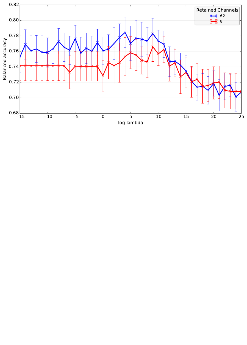
Figure 1: Mean performance traces (with standard error) of raxDAWN for 8 (red) and 62 (blue) retained pseudo channels

dependent on the regularization parameter (2

log lambda

3.2 Processing

The general processing scheme was taken from

ohrle et al., 2015). The open source software

pySPACE (Krell et al., 2013) was again used for im-

plementation. The data was cut into segments of one

second after the stimuli. For the ﬁrst noise cancel-

lation before the application of the spatial ﬁlter, we

performed a z-score standardization, decimation to

25 Hz, and a lowpass ﬁlter with a cutoff frequency

of 4 Hz. After the spatial ﬁlter, straight lines were ﬁt-

ted every 120 ms with a size of 400 ms and the slopes

were used as features. The features were standard-

ized again and the standard support vector machine

(SVM) from the LIBSVM package was used (Chang

and Lin, 2011). The SVM regularization constant was

optimized using a stratiﬁed 5-fold cross validation on

the training data

C ∈

, 10

−1

, . . . , 10

−5

. (20)

Finally the decision threshold was optimized. As per-

formance measure, we used the balanced accuracy

which is the arithmetic mean of true positive rate and

true negative rate.

For statistical tests, we used the Wilcoxon signed-

rank test.

3.3 Inﬂuence of the Regularization

For the ﬁrst evaluation, we only used the ﬁrst 24 ERPs

and the respective noise data from the irrelevant stim-

uli for training, since the regularization is expected to

pay off with few data.

In Figure 1, the effect of the regularization param-

eter λ is displayed for the case of no dimensionality

reduction (62 retained channels) and for the reduction

to the most relevant 8 pseudo channels

. To obtain a

substantial effect, λ should be chosen larger than 1.

The curves show ﬁrst an increase in performance due

to the regularization but then the performance drops

drastically because the regularization suppresses the

reduction of the noise and there is only a focus on

signal enhancement. Furthermore, the choice of λ is

very speciﬁc for the respective dataset and should be

optimized separately with a logarithmic scaling.

3.4 Inﬂuence of the Amount of Training

Data

If there is sufﬁcient data available, the algorithm is not

expected to overﬁt to much to the noise data. Hence

for a comparison between the ﬁlters the number of

used samples needs to be considered.

In this setting, we reduce the dimensionality to 8

pseudo channels and we compare the raxDAWN with

axDAWN and xDAWN for different numbers of train-

ing instances. The data was used till a predeﬁned

number of ERP samples have been reached in the

stream and the respective samples from the irrelevant

The large standard error results from the differences be-

tween the 10 evaluations (6 subjects with 2 recoding ses-

sion) and the different optimal λ values.

raxDAWN: Circumventing Overﬁtting of the Adaptive xDAWN

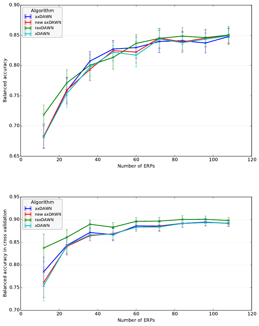
Figure 2: Comparison of spatial ﬁlters dependent on the number of training ERP samples (mean performance and standard

error).

Figure 3: Comparison of spatial ﬁlters dependent on the number of training ERP samples (mean performance and standard

error).

stimuli were used for the second class and the noise.

For optimizing λ, we used the same 5-fold cross vali-

dation as for the SVM regularization parameter C, but

with two repetitions to better ﬁlter out random effects

λ ∈

−5

, 2

−4

, . . . , 2

. (21)

So the optimization of the parameter seems a bit more

difﬁcult and dataset speciﬁc than the C parameter.

NEUROTECHNIX 2015 - International Congress on Neurotechnology, Electronics and Informatics

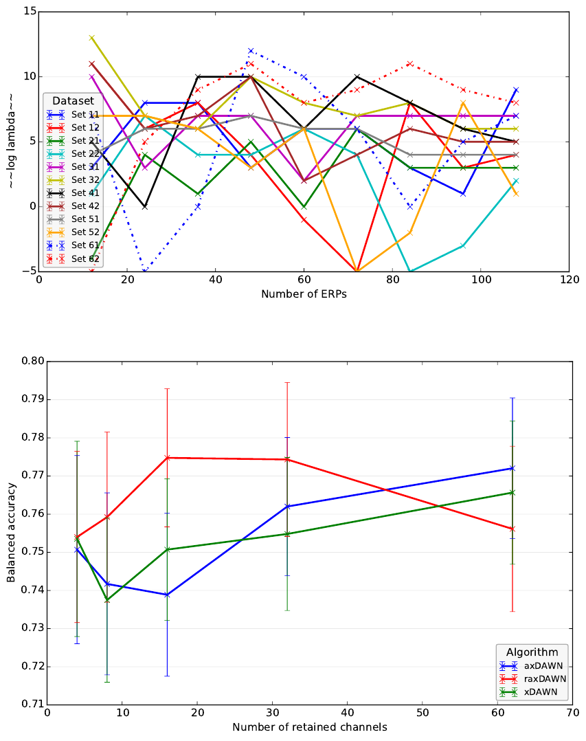
Figure 4: Lambda values chosen by the parameter optimization (2

log lambda

). The ﬁrst set index corresponds to the subject

number and the second index corresponds to the session number.

Figure 5: Comparison of spatial ﬁlters dependent on the number of retained channels (mean performance and standard error).

The results are shown in Figure 2. “New

axDAWN” denotes the raxDAWN with a small regu-

larization parameter of 2

−15

. As expected for all algo-

rithms, performances increase with increasing train-

ing size and axDAWN and xDAWN show approxi-

mately the same performance. Interestingly, the per-

formance of the “new axDAWN” is very close to the

xDAWN due to the improved initialization. If the

complete dataset is used for training, raxDAWN per-

forms similar to (a)xDAWN but for small sizes of the

raxDAWN: Circumventing Overﬁtting of the Adaptive xDAWN

training set (12 or 24 samples of the ERP class) it

clearly outperforms the other spatial ﬁlters by 4 or

1% (xDAWN: p = 0.009, aXDAWN: p = 0.003, and

new axDAWN: p = 0.02 for both numbers of sam-

ples). This result is expected, because for a larger

amount of the data the noise should not have such a

high inﬂuence anymore. Further, the result is con-

sistent with the ﬁndings in (Lotte and Guan, 2010),

where the highest performance increase due to regu-

larization of CSP was achieved when the amount of

available training data was very low.

In Figure 4, the chosen lambda values in the pa-

rameter optimization of the raxDAWN are shown.

The values are diverse and depend on the number of

used ERPs as well as on the dataset. This parame-

ter behavior is unexpected and needs further investi-

gation. A more sophisticated parameter optimization

might result in a more stable choice and even better

performance. The problem of parameter optimiza-

tion can be also observed when Figure 2 is compared

with Figure 3. Figure 3 displays the best performance

value in the cross validation cycle for the parameter

optimization. Here, the raxDAWN shows slightly bet-

ter performance in the cross validation for every num-

ber of used ERPs and not only for the low number.

This difference indicates a parameter overﬁtting.

3.5 Inﬂuence of the Number of Retained

Channels

In this evaluation, we used a reduced number of sam-

ples as in Section 3.3 but varied the number of re-

tained pseudo channels. Again the regularization pa-

rameter of the raxDAWN was optimized. The results

are shown in Figure 5. For a number of 4, there is no

large difference between the algorithms because the

noise has possibly less inﬂuence. For 62 channels the

raxDAWN performs slightly worse. For the group of

8, 16, and 32 retained channels, the raxDAWN outper-

forms the other ﬁlters by 1− 3% (xDAWN: p = 0.04,

axDAWN: p = 0.02). The other ﬁlters show no dif-

ference in performance (p = 0.49).

4 CONCLUSION

In this paper we successfully applied the regulariza-

tion concept for spatial ﬁlters to the axDAWN algo-

rithm and introduced the new raxDAWN algorithm.

We evaluated the algorithm on data from a BCI ex-

periment and showed that it improves xDAWN and

axDAWN especially in the initialization when only

few training data is available.

In the future, we would like to analyze other reg-

ularization methods. For example, the ﬁrst ﬁlter from

a previous session or a different subject could be used

for the regularization in a zero training setup instead

of using the ﬁlter for initialization as done in (W

ohrle

et al., 2015). Another point is a deeper analyses of

the optimal choice of the regularization parameter to

speed up the optimization. One possibility might be

an online optimization which combines some models

weighted by their accuracy.

ACKNOWLEDGEMENTS

This work was supported by the Federal Min-

istry of Education and Research (BMBF, grant no.

01IM14006A).

We thank Marc Tabie, Yohannes Kassahun and

our anonymous reviewers for giving useful hints to

improve the paper. We thank Su Kyoung Kim for pro-

viding the statistics.

REFERENCES

Blankertz, B., Lemm, S., Treder, M., Haufe, S., and M

uller,

K.-R. (2011). Single-Trial Analysis and Classiﬁca-

tion of ERP Components–a Tutorial. NeuroImage,

56(2):814–825.

Blankertz, B., Tomioka, R., Lemm, S., Kawanabe, M., and

uller, K.-R. (2008). Optimizing Spatial ﬁlters for

Robust EEG Single-Trial Analysis. IEEE Signal Pro-

cessing Magazine, 25(1):41–56.

Buttﬁeld, A., Ferrez, P. W., and Mill

an, J. d. R. (2006). To-

wards a robust BCI: error potentials and online learn-

ing. IEEE transactions on neural systems and rehabil-

itation engineering : a publication of the IEEE Engi-

neering in Medicine and Biology Society, 14(2):164–

Chang, C.-C. and Lin, C.-J. (2011). LIBSVM. ACM

Transactions on Intelligent Systems and Technology,

2(3):1–27.

Ghaderi, F. and Kirchner, E. A. (2013). Periodic Spa-

tial Filter for Single Trial Classiﬁcation of Event Re-

lated Brain Activity. In Biomedical Engineering, Cal-

gary,AB,Canada. ACTAPRESS.

Golub, G. H. and Van Loan, C. F. (1996). Matrix computa-

tions. Johns Hopkins University Press.

Kirchner, E. A., Kim, S. K., Straube, S., Seeland, A.,

ohrle, H., Krell, M. M., Tabie, M., and Fahle, M.

(2013). On the applicability of brain reading for pre-

dictive human-machine interfaces in robotics. PloS

ONE, 8(12):e81732.

Krell, M. M., Straube, S., Seeland, A., W

ohrle, H., Teiwes,

J., Metzen, J. H., Kirchner, E. A., and Kirchner, F.

NEUROTECHNIX 2015 - International Congress on Neurotechnology, Electronics and Informatics

(2013). pySPACE a signal processing and classiﬁca-

tion environment in Python. Frontiers in Neuroinfor-

matics, 7(40):1–11.

Krusienski, D. J., Sellers, E. W., Cabestaing, F., Bayoudh,

S., McFarland, D. J., Vaughan, T. M., and Wolpaw,

J. R. (2006). A comparison of classiﬁcation tech-

niques for the P300 Speller. Journal of neural engi-

neering, 3(4):299–305.

Liao, X., Yao, D., Wu, D., and Li, C. (2007). Combining

spatial ﬁlters for the classiﬁcation of single-trial EEG

in a ﬁnger movement task. IEEE transactions on bio-

medical engineering, 54(5):821–31.

Lotte, F. and Guan, C. (2010). Spatially Regularized Com-

mon Spatial Patterns for EEG Classiﬁcation. In 2010

20th International Conference on Pattern Recognition

(ICPR), pages 3712–3715.

Mika, S. (2003). Kernel Fisher Discriminants. PhD thesis,

Technische Universit

at Berlin.

Mika, S., R

atsch, G., and M

uller, K.-R. (2001). A mathe-

matical programming approach to the kernel ﬁsher al-

gorithm. Advances in Neural Information Processing

Systems 13 (NIPS 2000), pages 591–597.

Rao, Y. and Principe, J. (2001). An RLS type algorithm for

generalized eigendecomposition. In Neural Networks

for Signal Processing XI: Proceedings of the 2001

IEEE Signal Processing Society Workshop (IEEE Cat.

No.01TH8584), pages 263–272. IEEE.

Rivet, B., Souloumiac, A., Attina, V., and Gibert, G.

(2009). xDAWN Algorithm to Enhance Evoked

Potentials: Application to Brain-Computer Inter-

face. IEEE Transactions on Biomedical Engineering,

56(8):2035–2043.

Samek, W., Vidaurre, C., M

uller, K.-R., and Kawanabe, M.

(2012). Stationary common spatial patterns for brain-

computer interfacing. Journal of neural engineering,

9(2):026013.

van Erp, J., Lotte, F., and Tangermann, M. (2012). Brain-

Computer Interfaces: Beyond Medical Applications.

Computer, 45(4):26–34.

ohrle, H., Krell, M. M., Straube, S., Kim, S. K., Kirchner,

E. A., and Kirchner, F. (2015). An Adaptive Spatial

Filter for User-Independent Single Trial Detection of

Event-Related Potentials. IEEE transactions on bio-

medical engineering, PP(99):1.

ohrle, H., Teiwes, J., Krell, M. M., Kirchner, E. A., and

Kirchner, F. (2013). A Dataﬂow-based Mobile Brain

Reading System on Chip with Supervised Online Cal-

ibration - For Usage without Acquisition of Training

Data. In Proceedings of the International Congress on

Neurotechnology, Electronics and Informatics, pages

46–53, Vilamoura, Portugal. SciTePress.

Zander, T. O. and Kothe, C. (2011). Towards passive brain-

computer interfaces: applying brain-computer inter-

face technology to human-machine systems in gen-

eral. Journal of Neural Engineering, 8(2):025005.

raxDAWN: Circumventing Overﬁtting of the Adaptive xDAWN