
Software Implementation of Several Production Scheduling
Al
g
orithms
Vladimir Monov, Tasho Tashev and Alexander Alexandrov
Institute of Information and Communication Technologies, Bulgarian Academy of Sciences
Acad. G. Bonchev str., bl. 2, 1113 Sofia, Bulgaria
vmonov@iit.bas
.bg, ttashev@iit.bas.bg, akalexandrov@iit.bas.bg
Keywords: Scheduling algorithms, production schedules, manufacturing process.
Abstract: The paper presents several production scheduling algorithms and their software implementation in an
experimental program system developed in the program environment of the MATLAB system. The main
characteristics and functionality of the individual software modules are described and illustrated by
numerical examples.
1 INTRODUCTION
The theory of scheduling deals with problems for
optimal allocation of scarce resources for
implementation of various activities over time. One
broad class of scheduling problems involves the
dsign of production scheduling algorithms aimed at
the optimization of technological machine and
production capacity utilization in a production
process. Typically, such a process is characterized
by a number of jobs which have to be processed on a
number of machines or work places in a given order
or sequence. Depending on the specifics, scale and
complexity of the particular production process the
design of such schedules may represent a difficult
and intractable task. It is obvious, however, that the
use of optimal production schedules directly affects
the production process leading to reduced costs and
savings in energy and materials.
In this paper, we present a programme
implementation of six production scheduling
algorithms which are intended to solve some
frequently arising scheduling problems in the
production processes of small and medium
companies. The algorithms have been developed in
the course of a project supported by the National
innovation fund as a part of an experimental
programme system for production scheduling and
inventory control in small and medium enterprises.
2 MODELS OF SCHEDULING
PROBLEMS AND RELATED
WORK
We shall consider deterministic models of
scheduling problems where the number of jobs is
denoted by n and the number of machines by m.
Usually, the subscript j refers to a job while the
subscript i refers to a machine. The following
important data are associated with job j, (Pinedo,
2008).
Processing time (p
ij
) The p
ij
represents the
processing time of job j on machine i. The subscript
i is omitted if the processing time of job j does not
depend on the machine or if job j is only to be
processed on one given machine.
Release date (r
j
) The release date r
j
of job j may
also be referred to as the ready date. It is the time the
job arrives at the system, i.e., the earliest time at
which job j can start its processing.
Completion time (C
j
) This is the moment of
time at which the job j comes out of the system.
Clearly, the completion time of job j depends on the
jobs that have been processed before it.
Due date (d
j
) The due date d
j
of job j represents
the committed shipping or completion date (i.e., the
date the job is promised to the customer).
Completion of a job after its due date is allowed, but
then a penalty is incurred. When a due date must be
met it is referred to as a deadline and denoted by d
j
.
205
V. Monov V., Tashev T. and Alexandrov A.
Software Implementation of Several Production Scheduling Algorithms.
DOI: 10.5220/0005887202050212
In Proceedings of the Fifth International Symposium on Business Modeling and Software Design (BMSD 2015), pages 205-212
ISBN: 978-989-758-111-3
Copyright
c
2015 by SCITEPRESS – Science and Technology Publications, Lda. All rights reserved
Weight (w
j
) The weight w
j
of job j is basically a
priority factor, denoting the importance of job j
relative to the other jobs in the system. For example,
this weight may represent the actual cost of keeping
the job in the system. This cost could be a holding or
inventory cost; it also could represent the amount of
value already added to the job.
In the current literature it is commonly accepted
to describe a scheduling problem by the triplet < α |
β | γ >. The α field describes the machine
environment and contains just one entry. The β field
provides details of processing characteristics and
constraints and may contain no entry at all, a single
entry, or multiple entries. The γ field describes the
objective to be minimized and often contains a
single entry. Models of many scheduling problems
can be described in terms of the triplet < α | β | γ >,
e.g., see (Brucker, 2007, Pinedo, 2008).
We shall illustrate the usage of the above
notation by the following simple models.
• 1 | |
Σ C
j
denotes the model of a scheduling
problem where the jobs are processed on one
machine, no preemptions are allowed and the
objective is to minimize the sum of completion
times of all jobs.
• 1 | r
j
|
Σ C
j
denotes a variant of the above
problem where, in addition, release dates of the
jobs are specified indicating times at which jobs
can start their processing.
• 1 | r
j
, prmp, prec |
C
max
denotes the model
of a scheduling problem with one machine where
the jobs have release dates, their processing can
be interupted, there are precedence restrictions
and the objective is to minimize the processing
time of all jobs.
There are different types of schedules and one of
the first classification of various scheduling
problems can be found in the seminal work of
Conway et al., (1967). A comprehensive study of
scheduling algorithms and their complexity is
presented in Lawler et al., (1993). Deterministic
scheduling problems are considered in Graham et
al., (1979) and a survey of scheduling problems
subject to various constraints is given by Lee,
(2004). Special classes of scheduling problems with
penalties and non-regular objective functions are
considered by Baker and Scudder, (1990) and
Raghavachari, (1988). A survey of scheduling
problems with job families and problems with batch
processing, can be found in the work of Potts and
Kovalyov (2000). In the more recent literature,
production scheduling is also attracting a
considerable amount of research. A classification,
models and complexity results on problems for
parallel machine scheduling are given by (Edis et al.,
2013 and Prot et al., 2013). References (Allahverdi
et al., 2008), (Janiak et al., 2015) and (Kovalyov et
al., 2007) represent surveys on scheduling problems
with setup times, due windows and jobs with fixed
intervals, respectively. Tools for multicriteria
scheduling are desribed in (Hoogeveen, 2005) and
architectures of manufacturing scheduling systems
are discussed in (Framinan and Ruiz, 2010). Finaly,
it should be noted that the monographs (Brucker,
2007) and (Pinedo, 2008) give a systematic view of
the research work and advancement in the area of
scheduling theory and its applications.
3 GENERAL DESCRIPTION OF
THE PROGRAM SYSTEM
Our experimental software system is designed to
solve a number of problems arising in the
technological management of small and medium-
size enterprises. Two main groups of problems are
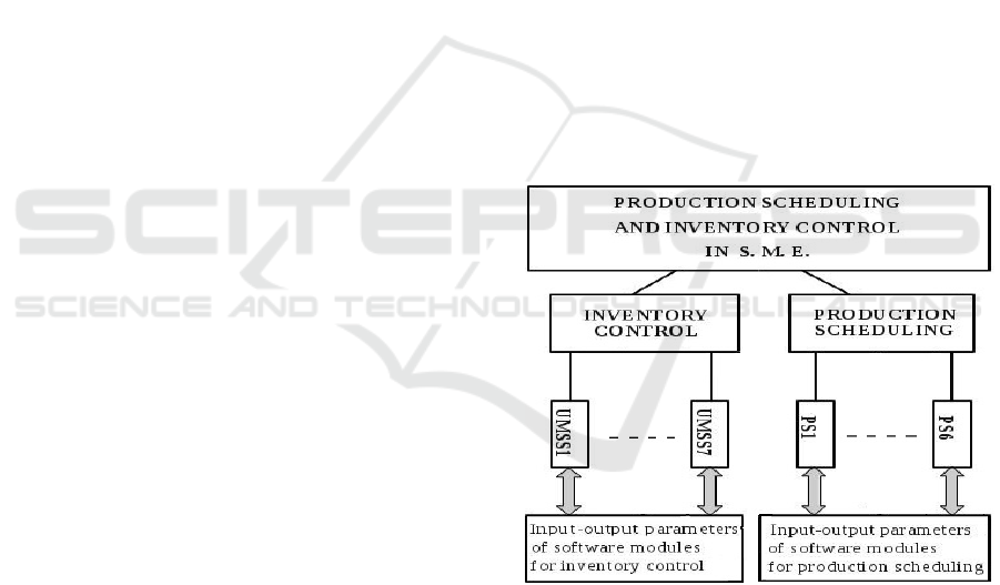
under consideration. The system architecture is
shown in Figure 1.
Figure 1: System architecture.
It is seen that it includes two main branches,
corresponding to the two groups of problems related
with inventory control and production scheduling,
respectively. Each branch in turn includes
algorithmic software modules to solve specific tasks
in the group. The programme system provides an
interactive mode of operation in which the user can
choose one of the two main branches and then starts
a specific algorithmic module depending on the
particular problem to be solved. In the process of
system operation, input-output parameters of the
Fifth International Symposium on Business Modeling and Software Design
206
system turn out to be input-output parameters of the
currently active module.
The description of program modules of UMSS1
to UMSS7 in Figure 1, as well as the specific tasks
to be solved by means of these modules were
presented in (Monov and Tashev, 2011). Program
modules from PS1 to PS6 will be described in the
next section.
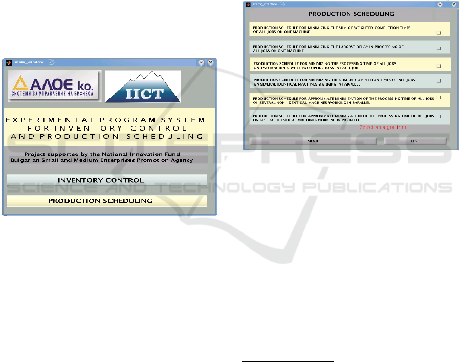
The graphical user interface of the system is
simplified and it includes three main modules:
main_window - interface module, bringing up
the main menu of the system;
start1_interface - interface module, displaying
the inventory control menu;
start2_interface - interface module displaying
the production scheduling menu.
The computer screen with the interface module
main_window is shown in Figure 2 and the launch
of this module in fact starts the system.
Figure 2: System main window.
By choosing one of the two groups of tasks, the
user can start the corresponding interface module
which displays the menu for choosing a particular
task to be solved. The computer screen of the
interface module displaying the production
scheduling menu is shown in Figure 3.
Each of the algorithmic software modules can
work within the program system and as an
independent module as well. In the second case it is
necessary the name of the module to be typed in the
command window of MATLAB. Then the
introduction of input data and the output of results is
accomplished by means of the system facilities of
the MATLAB programming environment. Each
module includes the following capabilities.
• Data input is performed in an interactive
mode from a standard keyboard, and the results
are displayed automatically after completing the
work of the algorithm.
• In each module, a check for correctness of
the input data is performed, an opportunity to
reintroduce incorrectly entered data is foreseen,
and also an opportunity is provided to exit the
module during data entry before the start of the
computational algorithm.
• Depending on the specifics of the particular
algorithm, the software module displays the
necessary messages concerning the problem
being solved.
• After completion of the work and upon a
request of the operator, input data and results can
be stored in a specified user file outside of the
system for further processing and analysis. The
name of this file is defined by the user.
Figure 3: Interface module start2_interface.
4 SOFTWARE MODULES FOR
PRODUCTION SCHEDULING
In this section, we briefly describe the scheduling
problems under consideration and illustrate the work
of the corresponding software modules intended to
solve these problems.
4.1 Production schedule for minimizing
the sum of weighted completion
times of all jobs on one machine -
Σ w
i
C
i
Problem formulation. The scheduling problem is
characterized by one machine environment, i.e. n=1
and m jobs. Each of these jobs has one operation
(consisting of a single operation), with processing
time p
j
. Clearly, in any random order of
implementation of the jobs, they will all be fulfilled
in time Σ p
j
. The completion times and weights of
the jobs are C
j
and w
j
, respectively. The problem
consists in finding such a sequence of jobs
processing which will minimize the weighted sum of
Software Implementation of Several Production Scheduling Algorithms
207
completion times of all jobs. Thus, the implemented
algorithm minimizes the quantity Σ w
i
C
i
.
Input data. These are: the number m of jobs, the
numbers p
j
>0 and numbers w
j
> 0.
Output data. This is the optimal schedule
indicating the sequence of processing of jobs that
will minimize the quantity Σ w
j
C
j
. The optimal
value of Σ w
j
C
j
is also computed.
The above problem is solved by means of the
software module PS1. The work of the module is
illustrated by the following numerical example.
Example 1. Consider the scheduling problem
with three jobs which have to be processed on one
machine with numerical data given in Table 1.
Table 1: Numerical data for Example 1.
Jobs, J
j
Processin
g
times,
p
j
Wei
g
hts, w
j
J
1
4 3
J
2
2 1
J
3
5 4
The software module PS1 computes the
quantities q
j
= p
j
/ w
j
, finds the optimal schedule and
the minimal value of Σ w
i
C
i
. The output results are
written in a user file which is given below.
_____________________________________________________
PRODUCTION SCHEDULE FOR MINIMIZING THE SUM OF
WEIGHTED COMPLETION TIMES OF ALL JOBS ON ONE
MACHINE - 1 | | Σ w
i
C
i
_____________________________________________________
_____________________________________________________
Optimal schedule
_____________________________________________________
_____________________________________________________
Job: 3
- Processing time (P
3
): 5
- Weight (W
3
): 4
- Value q = P
3
/ W
3
: 1.25
- Completion time (C
3
): 5
- Value (W
3
C
3
): 20
____________________________________________________
Job: 1
- Processing time (P
1
): 4
- Weight (W
1
): 3
- Value q = P
1
/ W
1
: 1.3333
- Completion time (C
1
): 9
- Value (W
1
C
1
): 27
____________________________________________________
Job: 2
- Processing time (P
2
): 2
- Weight (W
2
): 1
- Value q = P
2
/ W
2
: 2
- Completion time (C
2
): 11
- Value (W
2
C
2
): 11
_____________________________________________________
_____________________________________________________
Minimal value: Sum (WjCj) = 58
_____________________________________________________
4.2 Production schedule for minimizing
the largest delay in processing of all
jobs on one machine - 1 | | Lmax
Problem formulation. In this case, the objective is to
find an optimal schedule for the operation of one
machine under the following conditions. The
number of jobs to be processed is m and for each job
j two variables are given: the processing time p
j
and
the due date d
j
. All jobs are available at the initial
time and this allows them to be processed in any
order. If you choose such an order, then the job j will
be completed at the time C
j
and thus the delay of the
job is C
j
- d
j
. For any chosen order (sequence) of
processing, the delays of the jobs can be calculated.
Each particular order of jobs processing is
characterized by the maximum value among these
delays. The aim in this production scheduling
problem is to find this sequence of jobs processing
for which this maximum delay is as small as
possible.
Input data. These are: the number m of jobs, the
numbers p
j
>0 and numbers d
i
> 0.
Output data. This is the optimal schedule
indicating the sequence of processing of jobs that
will minimize the maximal delay L
max
of jobs. The
minimal value of L
max
is also computed.
The above problem is solved by means of the
software module PS2. The work of the module is
illustrated by the following numerical example.
Example 2. Consider the scheduling problem
with three jobs which have to be processed on one
machine with numerical data given in Table 2.
Table 2: Numerical data for Example 2.
Jobs, J
j
Processin
g
times,
p
j
Due dates, d
i
J
1
3 4
J
2
5 6
J
3
2 5
The software module PS2 computes the optimal
sequence of jobs processing which is <J
1,
J
3,
J
2
> and
the minimal value of L
max
which is L
max
= 4. For
comparison, if the jobs are processed in the order
<J
2,
J
3,
J
1
> then the corresponding delay is 6. The
output results are written in a user file which is
given below.
_____________________________________________________
PRODUCTION SCHEDULE FOR MINIMIZING THE
LARGEST DELAY IN PROCESSING OF ALL JOBS
ON ONE MACHINE - 1 | | LMAX
_____________________________________________________
_____________________________________________________
Fifth International Symposium on Business Modeling and Software Design
208
Optimal schedule
_____________________________________________________
_____________________________________________________
Job:
1
- Processing time (P
1
): 3
- Due date (D
1
): 4
- Completion time (C
1
): 3
- Delay C
1
-D
1
: -1
_____________________________________________________
_____________________________________________________
Job:
3
- Processing time (P
3
): 2
- Due date (D
3
): 5
- Completion time (C
3
): 5
- Delay C
3
-D
3
: 0
_____________________________________________________
_____________________________________________________
Job:
2
- Processing time (P
2
): 5
- Due date (D
2
): 6
- Completion time (C
2
): 10
- Delay C
2
-D
2
: 4
_____________________________________________________
The largest delay in the processing of jobs: C
2
-d
2
= 4
for job 2
__________________________________________
4.3 Production schedule for minimizing
the processing time of all jobs on
two machines with two operations
in each job F2 | | Cmax
Problem formulation. In this production scheduling
problem we have two machines which, in general,
are different. The number of jobs to be processed is
m and each of these jobs has two operations. For
each job the first operation is performed on machine
1 and lasts a
j
time units and the second operation is
performed on machine 2 and has a length b
j
. The
essential question in this problem is that for each job
the second operation can be run on a machine 2 only
after the complete implementation of the first
operation on the machine 1. It is necessary to find
such a sequence of jobs processing, in other words
to find such a schedule, at which the execution of all
the jobs is completed in the shortest time.
Input data. These are: the number m of jobs, the
processing times a
j
of the first operations and the
processing times b
j
of the second operations.
Output data. This is the optimal schedule
indicating the sequence of processing of jobs on the
two machines that will minimize the overall
processing time. The value of this time is also
indicated.
Remark. It should be noted that the optimal
sequence for the first machine is performed by
consecutively processing the first operations of the
jobs running on the machine immediately one after
another. The second operations of the jobs, however,
are executed on the second machine only after the
first operations has been completed on the first
machine.
The above problem is solved by means of the
software module PS3. The work of the module is
illustrated by the following numerical example.
Example 3. Consider the scheduling problem
with three jobs which have to be processed on two
machines with numerical data given in Table 3.
Table 3: Numerical data for Example 3.
Jobs, J
j
Processing times
a
j
of the first
operations on
Machine 1
Processing times b
j
of the second
operations on
Machine 2
J
1
4 1
J
2
2 5
J
3
6 3
The software module PS3 computes the optimal
sequence of jobs processing which is <J
2,
J
3,
J
1
> and
the minimal processing time of all jobs is 13. For
comparison, if the jobs are processed in the order
<J
1,
J
2,
J
3
> then the corresponding processing time is
15. The output results are written in a user file which
is given below.
___________________________________
PRODUCTION SCHEDULE FOR MINIMIZING THE
PROCESSING TIME OF ALL JOBS ON TWO MACHINES
WITH TWO OPERATIONS IN EACH JOB:
F2 || CMAX
_____________________________________________________
_____________________________________________________
Optimal schedule
_____________________________________________________
_____________________________________________________
Job:
2
- Processing time of operation 1 for this job: 2
- Processing time of operation 2 for this job: 5
_____________________________________________________
_____________________________________________________
Job:
3
- Processing time of operation 1 for this job: 6
- Processing time of operation 2 for this job: 3
_____________________________________________________
_____________________________________________________
Job:
1
- Processing time of operation 1 for this job: 4
- Processing time of operation 2 for this job: 1
__________________________________________
Minimum total execution time of all jobs : 13
_____________________________________________________
Software Implementation of Several Production Scheduling Algorithms
209
4.4 Production schedule for minimizing
the sum of completion times of all
jobs on several identical machines
working in parallel - P || Σ Cj
Problem formulation. The following production
scheduling problem is considered. There are n
identical machines working in parallel. The number
of jobs to be processed is m and each of these jobs
has one operation. The jobs processing times are p
j
.
For each job the processing time is the same for all
machines (identical machines). It is necessary to find
the optimal schedule which minimizes the sum of
completion times of all jobs.
Input data. These are: the number m of jobs, the
number n of machines, processing times p
j
.
Output data. This is the optimal schedule
indicating the particular jobs processing on each
machine and the sequence at which these jobs are
executed. The optimal value of the sum of
completion times ΣC j is also computed.
Remark. The implemented algorithm is based on
priorities and it uses the rule SPT (shortest
processing time first). The point is that all jobs are
ranked in order of monotonically increasing times p
j .
The first few jobs are distributed on the machines
and later, when a machine completes its work, the
next job is placed on this machine.
The above problem is solved by means of the
software module PS4. The work of the module is
illustrated by the following numerical example.
Example 4. Consider the scheduling problem
with seven jobs which have to be processed on three
machines with numerical data given in Table 4.
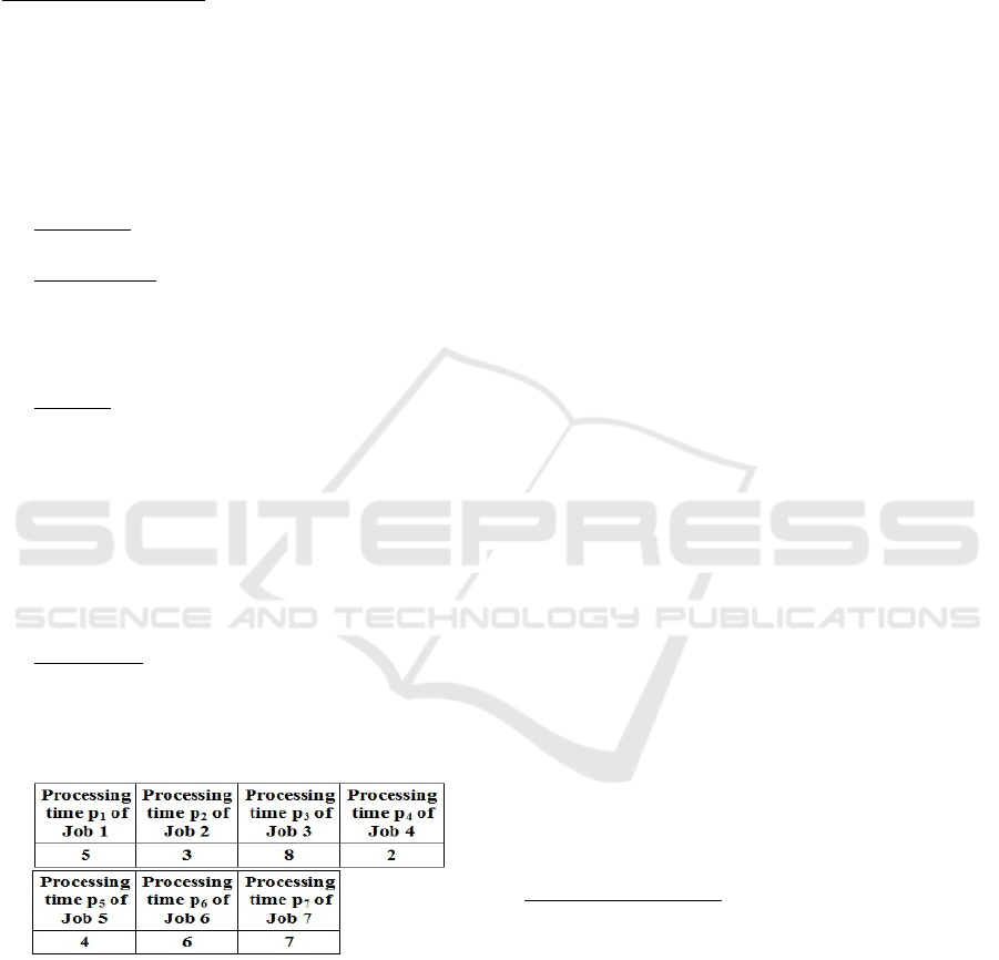
Table 4: Numerical data for Examples 4 and 6.
The software module PS4 computes the optimal
sequence of jobs processing on each machine and
the minimal value of the sum of completion times of
all jobs. This value is found to be 51. For
comparison, if the jobs are processed in the order
<J
1
,
J
2
,
J
3
,
J
4
, J
5
, J
6
, J
7
> then the corresponding value
of the sum is 58. The output results are written in a
user file which is given below.
_____________________________________________________
PRODUCTION SCHEDULE FOR MINIMIZING THE SUM OF
COMLETION TIMES OF ALL JOBS ON SEVERAL
IDENTICAL MACHINES WORKING IN PARALLEL
– P || Σ Cj
____________________________________________________
_____________________________________________________
Optimal Schedule
_____________________________________________________
Machine:1
_____________________________________________________
- Job:4
- Processing time of this job:2
_____________________________________________________
- Job:1
- Processing time of this job :5
_____________________________________________________
- Job:3
- Processing time of this job:8
_____________________________________________________
_____________________________________________________
Machine:2
_____________________________________________________
- Job:2
- Processing time of this job:3
_____________________________________________________
- Job:6
- Processing time of this job:6
_____________________________________________________
_____________________________________________________
Machine:3
_____________________________________________________
- Job:5
- Processing time of this job:4
__________________________________________
- Job:7
- Processing time of this job:7
_____________________________________________________
_____________________________________________________
Sum of completion times of all jobs:
Σ Cj :51
_____________________________________________________
4.5 Production schedule for
approximate minimization of the
processing time of all jobs on
several non-identical machines
working in parallel - Q || C
max
Problem formulation. There are several machines
which are not identical. This means that they have
different speeds of operation, but in all other aspects
of their capabilities are the same. A number of jobs
are to be processed, each of which consists of a
single operation. Any job can be executed on any
machine. The absolute speeds of operation of
machines are known in advance. The algorithm
calculates their relative speeds. The jobs processing
times on the slowest machine are known. All
machines and jobs are available at the initial time of
operation. The aim is to allocate jobs for execution
on machines in such a way as to obtain as little as
possible processing time of all jobs. The algorithm
Fifth International Symposium on Business Modeling and Software Design
210

gives approximate (suboptimal) solution of this
problem.
Input data. These are: the number of machines
and their absolute speeds of operation, the number of
jobs and their processing times on the slowest
machine.
Output data. The obtained schedule and the
processing time of all jobs.
Remark. The algorithm finds the relative speeds
of the machines and arranges them in order of
decreasing of these speeds. Then it arranges jobs in
order of decreasing of their individual processing
times on the slowest machine. The algorithm
allocates jobs on machines by putting the first of
waiting jobs on the fastest free (released) machine.
The above problem is solved by means of the
software module PS5. The work of the module is
illustrated by the following numerical example.
Example 5. Consider the scheduling problem
with five jobs which have to be processed on three
machines. The absolute speeds of operation are
given in Table 5 and the processing times of the jobs
on the slowest machine are given in Table 6.
Table 5: Absolute speeds of operation.
Machine 1 Machine 2 Machine 3
2 4 6
Table 6. Processing times.
Job 1 Job 2 Job 3 Job 4 Job 5
3 4 5 6 7
The software module PS5 computes a schedule
which approximately minimizes the processing time
of all jobs on the three machines. The output results
are written in a user file which is given below.
______________________
____________________
PRODUCTION SCHEDULE FOR APPROXIMATE
MINIMIZATION OF THE PROCESSING TIME OF
ALL JOBS ON SEVERAL NON-IDENTICAL MACHINES
WORKING IN PARALLEL - Q || Cmax
_____________________________________________________
_____________________________________________________
Computed schedule
_____________________________________________________
_____________________________________________________
Machine:3
-Relative speed of operation:3
-Total processing time of this machine:3.6667
_____________________________________________________
No1
Job:5
-Processing time of this job:2.3333
_____________________________________________________
No2
Job:2
-Processing time of this job:1.3333
_____________________________________________________
_____________________________________________________
Machine:2
-Relative speed of operation:2
-Total processing time of this machine:4.5
_____________________________________________________
No1
Job:4
-Processing time of this job :3
_____________________________________________________
No2
Job:1
-Processing time of this job:1.5
_________________________________________
_
___________
_____________________________________________________
Machine:1
-Relative speed of operation:1
-Total processing time of this machine:5
_____________________________________________________
No1
Job:3
-Processing time of this job:5
_____________________________________________________
Maximal processing time Cmax=5 obtained on machine:1
_____________________________________________________
4.6 Production schedule for
approximate minimization of the
processing time of all jobs on
several identical machines working
in parallel - P || C max
Problem formulation. In this production scheduling
problem there are m identical machines working in
parallel. The number of jobs is n and each of them
consists of one operation. The processing times of
jobs p
j
are known and for each job the processing
time is the same for all machines. The aim is to
allocate jobs for execution on machines in such a
way as to obtain as little as possible processing time
of all jobs. The algorithm gives approximate
(suboptimal) solution of this problem.
Input data. These are: the number of machines,
the number of jobs and their processing times.
Output data. The obtained schedule and the
processing time of all jobs.
Remark. The software module implements an
approximate algorithm using the LPT rule (longest
processing time first). At first all jobs are ranked in
order of monotonically decreasing times p
j
.
Observing the LPT rule, the first ordered jobs are
placed on the available machines. Next, as a
machine becomes free the next job is executed on it.
The algorithm enables us to estimate the deviation
from the optimal value of the problem. If we denote
by C max_opt the minimal processing time of all
jobs, then the implemented algorithm ensures
Software Implementation of Several Production Scheduling Algorithms
211

execution time, which is less than or equal to 4/3 C
max_opt. The above problem is solved by means of
the software module PS6. The work of the module is
illustrated by the following numerical example.
Example 6. Consider the scheduling problem
with seven jobs which have to be processed on three
machines. The jobs processing times are the same as
in Example 4 and are given in Table 4.
The software module PS6 computes a
suboptimal schedule including the following
sequence of jobs processing.
- Job3, Job2, Job4 are processed on Machine 1,
- Job7 and Job5 are processed on Machine 2,
- Job6 and Job1 are processed on Machine 3.
In this case the maximal processing time is C
max
=13
which is obtained on Machine 1.
5 CONCLUSIONS
The paper presents a software implementation of six
algorithms intended to provide solutions to some
basic production scheduling problems and to
facilitate the production management in small and
medium enterprises. Our experimental program
system is open for adding new modules and in a
future work, a library of scheduling algorithms and
software modules can be developed and
incorporated in the system. In particular, the system
capabilities can be extended by using more elaborate
mathematical models of manufacturing processes
taking into account various processing
characteristics and constraints and different machine
environments.
ACKNOWLEDGEMENTS
The research work reported in the paper is supported
by the project AComIn "Advanced Computing for
Innovation", grant 316087, funded by the FP7
Capacity Programme (Research Potential of
Convergence Regions).
REFERENCES
Allahverdi, A., C. T. Ng, T. C. E. Cheng, M. Y.
Kovalyov, 2008. A survey of scheduling problems
with setup times or costs, European Journal of
Operational Research 187, pages 985–1032.
Baker, K. R., G. D. Scudder, 1990. Sequencing with
Earliness and Tardiness Penalties: A Review,
Operations Research, 38, pages 22–36.
Brucker, P., 2007. Scheduling Algorithms, 5-th edition,
Springer.
Conway, R. W., Maxwell, W. L., Miller, L. W., 1967.
Theory of Scheduling, Addison-Wesley Publishing
Company, Massachusettts.
Edis, E. B., C. Oguz, I. Ozkarahan, 2013. Parallel machine
scheduling with additional resources: Notation,
classification, models and solution methods, European
Journal of Operational Research 230, pages 449–463.
Framinan, J. M., Rubén Ruiz, 2010. Architecture of
manufacturing scheduling systems: Literature review
and an integrated proposal, European Journal of
Operational Research 205, pages 237–246.
Graham, R. E., E. L. Lawler, J. K. Lenstra, A. H. G.
Rinnooy Kan, 1979. Optimization and approximation
in deterministic sequencing and scheduling: a survey,
Annals of Discrete Mathematics, 4, pages 287-326.
Hoogeveen, H., 2005. Multicriteria scheduling, European
Journal of Operational Research, 167, pages 592–623.
Janiak, A., W. A. Janiak, T. Krysiak, T. Kwiatkowski,
2015. A survey on scheduling problems with due
windows, European Journal of Operational Research,
242, pages 347–357.
Kovalyov, M. Y., C. T. Ng, T. C. Edwin Cheng, 2007.
Fixed interval scheduling: Models, applications,
computational complexity and algorithms, European
Journal of Operational Research, 178, pages 331–342.
Lawler, E. L., J. K. Lenstra, A. H. G. Rinnooy Kan and D.
Shmoys, 1993. Sequencing and Scheduling:
Algorithms and Complexity, in Handbooks in
Operations Research and Management Science, Vol.
4: Logistics of Production and Inventory, S. S. Graves,
A. H. G. Rinnooy Kan and P. Zipkin, (eds.), North-
Holland, New York, pages 445-522.
Lee, C. Y., 2004. Machine Scheduling with Availability
Constraints, Chapter 22 in Handbook of Scheduling, J.
Y.-T. Leung (ed.), Chapman and Hall/CRC, Boca
Raton, Florida.
Monov, V., T. Tashev, 2011. A programme
implementation of several inventory control
algorithms, Cybernetics and Information
Technologies, 11, pages 64-78.
Pinedo, M., 2008. Scheduling: Theory, Algorithms and
Systems, 3-rd edition, Springer.
Potts, C. N., M. Y. Kovalyov, 2000. Scheduling with
Batching: A Review, European Journal of Operational
Research, 120, pages 228–249.
Prot, D., O. Bellenguez-Morineau, C. Lahlou, 2013. New
complexity results for parallel identical machine
scheduling problems with preemption, release dates
and regular criteria, European Journal of Operational
Research, 231, pages 282–287.
Raghavachari, M., 1988. Scheduling Problems with Non-
Regular Penalty Functions: A Review, Opsearch, 25,
pages 144–164.
Fifth International Symposium on Business Modeling and Software Design
212
