
Two Phases Inventory Strategy of Non-instantaneous Deteriorating
Yao Chun and Sun Jianhong
*
School of Business, Ningbo University, NO.818,Fenghua Road, Ningbo, China
Yaochun1992@126.com, sunjianhong @nbu.edu.cn
Keywords: Fresh Agricultural Products, Non-instantaneous Deteriorating, Two Phases, Inventory Strategy.
Abstract: In this paper, we consider a replenishment model to maximize the average profits of fresh agricultural
products would not immediately deterioration. The paper discuss in a replenishment cycle, demand affected
only by fresh agricultural products price during “fresh-keeping period”, and during “period of
deterioration”, demand affected by freshness and fresh agricultural products price. Numerical examples are
included for illustration. The results show that decrease the rate of deterioration of fresh agricultural
products would be increase the average profits of system and when T=22, the total profits and the average
profits of the optimal.
*
Corresponding author
Fund Project: (project number: kg2013098) results; (project number: 13HYJDYY03 ) results; (project number: 15FJY005)
results; (project number: JGZDI201204) results.
1 INTRODUCTION
With the socioeconomic development and people's
lifestyle change, more and more urbanites begin to
pay attention to healthy eating and seasonal products
are quickly becoming the top choice among them. It
may be observed that the price of fresh agriculture
product is no longer the only factor for urbanite's
purchase, and the freshness becomes another
important measurable indicator for their purchase
decision. The fresh agriculture product is a kind of
seasonal and fresh product which has a relatively
short life cycle and liable to quick deterioration, such
as vegetables, fruits, and seafood. It is a special
perishable and vulnerable product that still has life
activities or similar animate in a state of inventory.
The demand for fresh agriculture product was easily
affected by freshness because random life cycle.
Consumers can get information of freshness by their
sensory modalities after fresh agriculture product on
hangers and we call this the sensory recognition
method. Despite the freshness of fresh agriculture
product will decay with the passing of time, there are
time node for consumers' perceive of the fresh to old.
Although it has lost its minor value in short time
after fresh agriculture product on hangers, perceived
the change is difficult for consumers. Fresh
agricultural products would not immediately
deterioration and this change process we call it
“fresh-keeping period”. During this time, the demand
is only affected by price, both price and freshness are
considered after this time node. This paper is
focused on the study of different influence factors of
demand in the same replenishment epochs, and it
will be meaningful for retailers to adjust fresh
agricultural product reasonable prices and make
reasonable replenishment decision.
The rest of the paper is organized as follows. In
the next section, we briefly discuss the current
literature and the contributions of this paper. Section
3 is devoted to the assumptions of the modeling
framework. The formulations and numerical
examples are presented in section 4 and section 5.
Section 6 is the paper’s conclusion.
2 LITERATURE
Dan (2008) and Chen (2009) discussed fresh
agricultural product supply chain coordination
problem under valuable loss and physical loss, using
an exponential function with downward slope, trying
to denote valuable loss with greenness. Wang and
Chen (2012) introduced the options contracts into
73
Jianhong S. and Chun Y.
Two Phases Inventory Strategy of Non-instantaneous Deteriorating.
DOI: 10.5220/0006019300730077
In Proceedings of the Information Science and Management Engineering III (ISME 2015), pages 73-77
ISBN: 978-989-758-163-2
Copyright
c
2015 by SCITEPRESS – Science and Technology Publications, Lda. All rights reserved
73

the fresh produce supply chain ordering decision
models, and the huge circulation wastages both from
quantity and quality were taken into account the two
stage models in one period. The paper supposed that
the demand would be affected by the produce’s fresh
degree. Lin et al. (2011) constructed a new
logarithmic freshness function and then told that the
revenue-sharing contract have an influence on supply
chain coordination under the time constraints. All of
the paper considered freshness would affect demand.
In addition, other scholars considered that the
demand would be affected by price and fresh .Chen
et al. (2009) developed a deteriorating inventory
model with freshness in consideration and the
demand depends on freshness and retail price
inventory model is established. Then, an ordering
policy of fresh agricultural products is studied under
elastic demand, progressive price discount and loss-
controlling. Gan et al. (2013) developed a demand
function influenced by the freshness and price of the
fresh agricultures product. Loss-averse utility
function and dynamic no-cooperative game theory
are applied in the model to discuss cooperation of
fresh products supply chain in E-commerce. Wang
and Dan (2013) according to the characteristics of
freshness decrease over time of the fresh agricultural
product, a time-varying consumer choice model
influenced by the freshness and price of the fresh
agricultures product is developed. In addition, a
multi-item ordering model for various fresh
agricultural products is developed to analyze the
retailer’s ordering policies under different unit fresh
keeping cost of supplier. Yan et al. (2014)
considered the coordination of a three-level fresh
agricultural product supply chain under
internet .Demand affect by price and freshness and
built the distribution of profits model based on the
improved revenue-sharing contract.
However, the above literatures either consider
demand affected by price or price and freshness in a
replenishment cycle. In real life, however, due to the
particularity of consumer awareness, in the early
stage of the fresh produce consumer perception of
product freshness basic convergence. So this paper
analyses the demand influence by different factors in
two phases in a replenishment cycle.
The paper consider in a replenishment cycle,
demand affected only by fresh agricultural products
price during “fresh-keeping period” and during
“period of deterioration”, demand affected by
freshness and fresh agricultural products price. In
this view, this article trying to build different pricing
model of two stages of fresh agricultural products
demand function, so as to provide theory for retailers
to scientific and rational pricing reference.
3 MODELING ASSUMPTIONS
AND NOTATION
Assumption 1:
(1) retailers instantaneous replenishment, lead
time is zero.
(2) this paper reference literature
[9]
about the
structure of the fresh degree function and make a
little change. The attenuation function for freshness
is θ(t)=θ
0
e
-ηt
, θ
0
is initial freshness of fresh
agricultural products, η is attenuation coefficient of
freshness (0<η<1).
(3) When 0<t<t
1
, demand function is D
1
(t)=a
1
-
b
1
p
1
. When t
1
<t<T, Demand function is D
2
(t)=a
2
-
b
2
p
2
+cθ(t). a
i
is market capacity, b
i
is price elasticity
(0<b
1
<b
2
). c means the coefficient of the fresh
agricultural product freshness to demand.
(4) when t belongs to (0,t
1
), the paper called it
“fresh-keeping period”. Fresh agricultural products
would not immediately deterioration, so demand
affected only by fresh agricultural products price.
When t belongs to (t
1
,T), the paper called it “period
of deterioration”. Demand affected by freshness and
fresh agricultural products price.
In the rest of the paper, the following notation is
used: p
1
denotes the price of fresh agricultural
product of fresh-keeping period, p
2
denotes the price
of fresh agricultural product of period of
deterioration. I(t) is the retail’s inventory level of
time t. T means replenishment cycle, Q denotes
order quantity of single cycle, A means fixed costs of
single cycle. PC is purchasing cost , Cp is unit
purchase of the item , HC is holding cost , h is unit
holding cost, DC is deterioration cost, Cd is unit
deterioration cost, SR denotes the total sales
revenue, TP denotes total profits, AP means average
profits. λ is deteriorating rate, θ
0
is initial freshness
of fresh agricultural products, η is attenuation
coefficient of freshness (0<η<1). a
i
is market
capacity, b
i
is price elasticity (0<b
1
<b
2
). c means the
coefficient of freshness to demand.
ISME 2015 - Information Science and Management Engineering III
74
ISME 2015 - International Conference on Information System and Management Engineering
74
4 MODEL FORMULATION AND
SOLUTION
4.1 Model Formulation
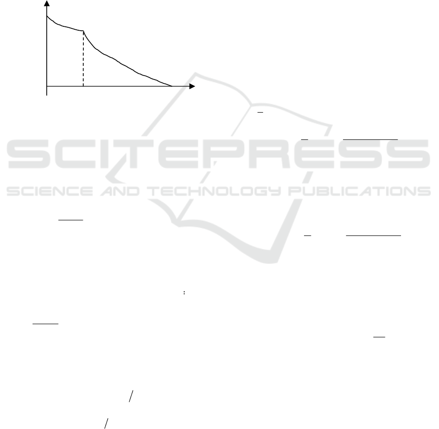
As is shown in fig1, the initial inventory level is Q.
When 0<t<t
1
, demand affected only by fresh
agricultural products price and demand function is
D
1
(t)=a
1
-b
1
p
1
. When t
1
<t<T, demand affected by
freshness and fresh agricultural products price.
Demand function is D
2
(t)=a
2
-b
2
p
2
+cθ(t).
Figure 1: Fresh agricultural products two-phase inventory
chart.
When 0<t<t
1
, fresh agricultural products would
not immediately deterioration.
Inventory level is only affected by demand.
Inventory level I
1
(t) satisfied:
(
)
1
1 1 1
( )
dI t
D a b p
dt
= − = − −
(1)
The boundary conditions I
1
(0)=Q, so solving
equation (1), the Inventory level I
1
(t):
(
)
1 1 1 1
( )
I t a b p t Q
= − − +
(2)
When t
1
<t<T ,inventory level I
2
(t) satisfied
(
)
( )
2
2 2 2 2
( c (t))
dI t
a b p I t
dt
θ λ
= − − + −
(3)
The boundary conditions I
2
(t)=0, solving
equations (3):
(
)
( ) T
2
( )
t T t
I t A Be Ae Be e
η λ λ η λ
− − −
= − − + +
(4)
2
2 2
( )
A a b p
λ
= −
(5)
0
( )
B c
θ λ η
= −
(6)
By the function of continuity, we know I
1
(t)=
I
2
(t), solving equations (2)and (4), We know the
function relation between order quantity and
replenishment cycle
(
)
1 1
( ) T
1 1 1 1
( )
t tT
Q A Be Ae Be e a b p t
η λλ λ η
− −−
= − − + + + −
(7)
Therefore , in a replenishment cycle T, all of the
cost and profits as follows:
1)The cost of the fixed order: A
(8)
2) Purchasing Cost : PC
( )
1 1
( ) T
1 1 1 1
( )
p
t tT
p
PC C Q
C A Be Ae Be e a b p t
η λλ λ η
− −−
=
= − − + + + −
(9)
3) Holding Cost : HC
( )
1
1
1 1
1 2
0
2
1 1 1 1 1
( )
( ) ( )
1
(t)dt (t)dt
1
2
( )
t T
t
T T
T t T t
HC h I h I
a b p t Qt
h
B Ae Be
A T t e e
λ λ η
η λ
η λ
−
− − − −
= ⋅ + ⋅
− + + +
= ⋅
+
− − + − ⋅
∫ ∫
(10)
4) Deterioration Cost: DC
1
1 1
2
( )
( ) ( )
1
(t)dt
( )
T
d
t
T T
T t T t
d
DC C I
B Ae Be
C A T t e e
λ λ η
η λ
λ
λ
η λ
−
− − − −
= ⋅
+
= − − + − ⋅
∫
(11)
5) Sales Revenue: SR
[ ]
( ) ( )( )
( )
1
1
1
1
1
1 1 2 2
0
1 1 1 1 2 2 2 2
0
0
1 1 1 1 1 2 2 2 2 1
(t) (t)
( ) ( )
t T
t
t T
t
tT
SR p D dt p D dt
p a b p dt p a b p c t dt
c
p a b p t p a b p T t e e
ηη
θ
θ
η
−−
= +
= − + − + ⋅
= − + − − − −
∫ ∫
∫ ∫
(12)
6) Total Profits : TP
T t
1
0
Q
Two Phases Inventory Strategy of Non-instantaneous Deteriorating
75
Two Phases Inventory Strategy of Non-instantaneous Deteriorating
75

( ) ( )( )
( )
( )
( )
1
1 1
1
1
0
1 1 1 1 1 2 2 2 2 1
( ) T
1 1 1 1
( )
1
2
1 1 1 1 1
( )
( )
( )
( )
( )
1
2
tT
t tT
p
T t
T T
T t
TP SR A PC HC DC
c
p a b p t p a b p T t e e
A C A Be Ae Be e a b p t
B
A T t e
h a b p t Qt
Ae Be
e
ηη
η λλ λ η
η
λ λ η
λ
θ
η
η
λ
−−
− −−
− −
−
− −
= − + + +
− + − − − − −
+ − − + + + − +
=
− − + −
⋅ − + + +
+
⋅
1 1
( )
( ) ( )
1
( )
T T
T t T t
d
B Ae Be
C A T t e e
λ λ η
η λ
λ
η λ
−
− − − −
+
+
− − + − ⋅
(13)
7) Average Profits : AP
TP
AP
T
=
(14)
And
(
)
2
1 1 1 1 1 1 1 1 1 1
2 (1/ 2)
p
AP p a t b t p C t b hb t
∂ ∂ = − + −
(15)
( )
( )
( )
( )
1
1 1
1
0
2 2 2 1
2
( )
2 2 2
1
2
2 2
1
2
( 2 )( )
1
tT
T t t
p
t
d
c
AP
a b p T t e e
p
b b b
C e h T t e
b b
C T t e
ηη
λ λ
λ
θ
η
λ λ λ
λ
λ λ
−−
−
∂
= − − − − −
∂
⋅ − + − +
+ − +
(16)
4.2 Model Solution
Theorem1: The fresh agricultural products profits
model has the optimal solution .
Proof: 1) The necessary condition of the optimal
solution is to find p
1
* and p
2
* that can satisfy Partial
derivative is zero.
(
)
2
1 1 1 1 1 1 1 1 1
2 (1/ 2) 0
p
a t b t p C t b hb t
− + − =
(17)
( )
( )
( )
( )
1
1 1
1
0
2 2 2 1
( )
2 2 2
1
2
2 2
1
2
( 2 )( )
1
0
tT
T t t
p
t
d
c
a b p T t e e
b b b
C e h T t e
b b
C T t e
ηη
λ λ
λ
θ
η
λ λ λ
λ
λ λ
−−
−
− − − − −
⋅ − + − +
=
+ − +
(18)
Solving equations (17) and (18), we know
*
1 1 1 1
1 2 (1/ 2)
p
p ht C a b
= − + +
(19)
( )
(
)
( ) ( )
( )
1
1
1
( )
2
*
2
1
2
2 1 2
0
1
1
1
2 2
T t
p
t
d
t
T
C e
b
a
T t e h C
p
b T t b
c
e e
λ
λ
η
η
λ
λ
λ
θ
η
−
−
−
− +
− + +
= +
− −
+ −
(20)
So, there are p
1
* and p
2
* that can satisfy the
necessary condition of optimal solution.
According equations (15) and (16), the partial
derivatives of p
1
and p
2
are as follows:
2 2
1 1 1
2 0
AP p b t
∂ ∂ = − <
(21)
2 2
2 2 1
2 ( ) 0
AP p b T t
∂ ∂ = − − <
(22)
2 2
1 2 2 1
0
AP p p AP p p
∂ ∂ ∂ = ∂ ∂ ∂ =
(23)
The Hessian matrix is
1 1
2 1
2 0
0 2 ( )
b t
H
b T t
−
=
− −
(24)
2
2 2 2
2 2
1 2 1 2
0
AP AP AP
H
p p p p
∂ ∂ ∂
= − >
∂ ∂ ∂ ∂
(25)
Solving equations (21) to (25), the Hessian
matrix negative, the maximum profits function
exists.
5 NUMERICAL EXAMPLES AND
SENSITIVITY ANALYSIS
Table 1 shows the Optimal prices, the optimal order
quantity, expected revenues, in that order, for
different values of T and for given value of a
1
, a
2
, b
1
,
b
2
, c, λ, η, θ
0
, h, Cp, Cd. And a
1
=120, a
2
=100, b
1
=8,
b
2
=15, c=100, λ=0.1, η=0.2, θ
0
=0.9, h=0.05, Cp=3,
Cd=0.1.
ISME 2015 - Information Science and Management Engineering III
76
ISME 2015 - International Conference on Information System and Management Engineering
76

Table 1: For different values of T.
T* P
1
* P
2
* Q* TP* AP*
24 8.9 4.312 1011 4181.668 174.237
22 8.9 4.795 1086 4447.149 202.143
20 8.9 5.250 1047 3865.08 193.254
18 8.9 5.724 988 3350.61 186.145
From table 1 we see the following conclusion:
(1) As T* increase, the price of p
2
* decrease. p
2
represents the price of fresh agricultural product of
period of deterioration. With the increase of T*,
fresh agricultural products constantly deterioration
and of course price falling.
(2) As T* increase, the order quantity gradually
increasing firstly. And when T=22, the order
quantity at its highest point. When ordering quantity
reaches a certain extreme value point, the fresh
agricultural products accelerate deterioration if
continue to extend the ordering cycle.
(3) As T* increase, the average profits increase
and decrease trend is the same as the order quantity.
Table 2 shows: for different values of η* and for
given value of a
1
, a
2
, b
1
, b
2
, c, λ, θ
0
, h, Cp, Cd. T
And a
1
=120, a
2
=100, b
1
=8, b
2
=15, c=100, λ=0.1,
η=0.2, θ
0
=0.9, h=0.05, Cp=3, Cd=0.1, T=22.
Table 2: For different values of η*.
η* P
1
* P
2
* Q* TP* AP*
0.2 8.9 4.795 1086 4447.149 202.143
0.4 8.9 4.708 1023 4318.116 196.278
0.6 8.9 4.621 960 4186.116 190.413
0.8 8.9 4.534 897 4060.056 184.584
From table 2 we see that as η* increase, P
2
*
decrease, Q* decrease, AP* also decrease. Because
θ(t) is a decreasing function and for fresh
agricultural products , the higher the deterioration
rate , the lower the price.
6 CONCLUSIONS
The paper considered the demand affected by
different factors of two phases inventory
replenishment. Due to the characteristics of non-
instantaneous deteriorating of fresh agricultural
products and the particularity of consumer
perception, demand affected only by fresh
agricultural products price during “fresh-keeping
period”, and during “period of deterioration”,
demand affected by freshness and fresh agricultural
products price. Numerical examples are included for
illustration. The conclusion is as follows: (1) when
T=22, total profits and average profits maximum; (2)
the faster the decline rate, the lower the price of P
2
*
and at the same time, order quantity, total profits and
average profits decrease.
However, in this paper we assuming that
replenishment lead time is zero, in real life, out of
stock is frequent and it is a real important problem
for retailer. So the article also can construct the
model from the order lead time is not zero, retailers
allow delayed payment etc.
REFERENCES
Dan Bin, Chen Jun. 2008. Coordinating Fresh Agricul
tural Supply Chain under the Valuable Loss. Chin
ese Jour-nal of Management Science. 2008,05:42-4
9.
Chen Jun ,Dan Bin. 2009. Fresh agricultural product
supply chain coordination under the physical loss-
controlling. Systems Engineering-Theory&Practice.
03:54-62.
Wang Jing, Chen Xu. 2011. Fresh produce supplier’s
pricing decisions research with circulation wastag
e and options contracts. Forecasting. 05:42-47.
Lin Lue, Yang Shuping. 2011. Three-level Supply Ch
ain Coordination of Fresh Agricultural Products wi
th Time Constraints. Chinese Journal of Managem
ent Science.03:55-62.
Chen Jun , Dan Bin. 2009. EOQ model for fresh agr
icultural product under progressive price discount
and loss-controlling. Systems Engineering-Theory&
Practice. 07:43-54.
Gan Xiaobing, Qian Liling. 2013. Coordination and o
ptimization of two-tiered fresh products supply cha
in in E-commerce. Journal of Systems & Manage
ment. 05:655-664.
Wang Lei, Dan Bin. 2013. A multi-item ordering mo
del for fresh agricultural products with time-varyin
g customer utility affected by freshness. Journal of
Systems & Management. 05:647-654.
Yan Bo, Ye Bing, Zhang Yongwang. 2014. Three-lev
el supply chain coordination of fresh agricultural
products under internet of things. Systems Enginee
ring.01:48-52.
Ding Song, Dan Bin. 2012. Optimal ordering policy f
or fresh agricultural products with stochastic dema
nd considering retailers’ risk preference. Chinese J
ournal of Management Science. 09:1382-1387.
Two Phases Inventory Strategy of Non-instantaneous Deteriorating
77
Two Phases Inventory Strategy of Non-instantaneous Deteriorating
77
