A Comparative Analysis of Pickup Forecasting Methods for Customer

Arrivals in Airport Carparks

Andreas Papayiannis, Paul Johnson and Peter Duck

School of Mathematics, University of Manchester, Manchester, U.K.

Keywords:

Lead Time, Booking Curve, Pick Up.

Abstract:

Accurate forecasts of customer demand lie at the core of any successful revenue management system. Most

research has focused upon studying such methods for the airline and hotel industry. In this paper, we present a

comparative analysis of various forecasting methods which we apply to the rapidly evolving airport carparking

(ACP) industry. We use real ACP booking data from four distinct carparks of a major airport in UK to forecast

customer arrivals for one to eight weeks out in the future. Conclusions are reached with regards to which

forecasting methods perform best in this operating environment, and whether there is any beneﬁt in employing

complex methods over simpler ones.

1 INTRODUCTION

Accurate forecasts of customer demand lie at the core

of any successful revenue management (RM) system,

as several reports point out a signiﬁcant further in-

crease on generated revenues. In particular, for the

airline industry (Lee, 1990) shows that a 10% im-

provement in forecasting accuracy can result in up to

3% increase on revenues, while in hotels a 20% fore-

casting improvement leads to 1% revenue increase

olt, 1998). As a result, several studies on forecast-

ing methods have been presented; a good review on

these methods may be found in (Sa, 1987) and (Lee,

1990) for the airlines and (Weatherford et al., 2001),

(Weatherford and P

olt, 2002) and (Weatherford and

Kimes, 2003) for hotels.

In carparks, the forecasting requirements and

models are closely related to those in the hotel indus-

try. One such study refers to the masters thesis of

(Rojas, 2006) who developed a neural network model

to forecast demand on an hourly basis and compared

it against some traditional historical time-series mod-

els. His results indicate that the ability of the neural

network method to capture the demand changes from

high to low periods improves performance accuracy.

In airport carparks, the setting is similar; multi-

ple carparks are located around the airport and people

choose among them based on their intended duration-

of-stay, proximity to the airport and price. Over the

last decade, the implementation of online reserva-

tion systems for airport carparks has gained interest,

with all major airports in UK and Europe offering

online pre-booking through their ofﬁcial websites as

well as through third parties. This enabled managers

to use traditional RM techniques to forecast demand

per length-of-stay (LoS) and per rate category offered

(product) in a each carpark.

According to (Weatherford and Kimes, 2003) RM

forecasting methods fall into three main types:

• Historical booking models

they only consider the ﬁnal number of arrivals on

a given day in history

• Booking curve (pickup) models

they take into account the booking build-up pat-

tern of arrivals during the lead time

• Combined models

they combine historical and booking curve models

using either a weighted average or regression, to

develop better forecasts.

In this paper, we use real ACP booking data from

four distinct carparks of a major airport in UK to

forecast customers arrivals. Normally, such forecasts

are fed into the optimization routines to drive capac-

ity or pricing decisions. Consequently, this piece of

work comes as a pre-requisite for the revenue opti-

mization algorithms developed in (Papayiannis et al.,

2012; Papayiannis et al., 2013) for ACP. Our aim is

to provide a comparative analysis of various forecast-

ing models and make valid conclusions on balancing

between a method’s simplicity and accuracy. Moti-

vated by the results presented in (Wickham, 1995) for

Papayiannis, A., Johnson, P. and Duck, P.

A Comparative Analysis of Pickup Forecasting Methods for Customer Arrivals in Airport Carparks.

DOI: 10.5220/0005631900150024

In Proceedings of 5th the International Conference on Operations Research and Enterprise Systems (ICORES 2016), pages 15-24

ISBN: 978-989-758-171-7

the airline industry, where the booking curve methods

were found in general to be the most accurate, we re-

strict our focus to these type of methods. Three main

attributes shape up the exact type of the pickup vari-

ation to be used; the ﬁrst two control the structure of

the pickup method while the third refers to the under-

lying time-series model. In a similar study, (Zakhary

et al., 2008) tested the resulting pickup variations, us-

ing simulated hotel data, for two models; the mov-

ing average and the exponential smoothing model.

Our work implements the same structural methodol-

ogy, but it also extends further to cover more complex

time-series models that account for seasonality and/or

autocorrelation in the data. Consequentially, in order

to describe the pickup methodology and its variations

we ﬁnd it convenient to use similar notation.

In section 2, we introduce and describe the pickup

methodology, its structural variations and the time-

series models under study. Further, we design a cross-

validation procedure to recursively obtain forecasts as

time unfolds and deﬁne the three performance mea-

sures that are used to assess the accuracy of the meth-

ods. The best models are selected based on all three

measures. Finally, results of our analysis are found in

section 3 while conclusions on the best practices as

well as further work are summarised in section 4.

2 BACKGROUND

Booking curve models are quite popular in practice

because they are intuitive and easy to set up. Their

special feature is that they use the build-up pattern

of reservations of past days, as opposed to only their

complete arrival histories. In general, booking build-

up models forecast total arrivals on a future day T by

estimating the bookings-to-come between now and T .

They are often called pickup models as they estimate

reservations to be picked up from a given point in time

to a different point in time during the booking process

(Zakhary et al., 2008).

Table 1 shows the evolution of customer demand

in a matrix form. Each row represents the booking

build-up of arrivals for each arrival date in August.

More precisely, each column on the right hand side is

a snapshot of on-hand bookings for the given arrival

day on the left, as of some lead time. Seven review

points are shown, on the day, one day in advance, two

days in advance up to six days in advance. Let us

assume that today’s date is the 9

of August. Then,

the number of total arrivals on, say, the 6

of August

was 234, where 190 of them had booked four days and

more in advance (they had already booked by the 2

of August). For arrival dates that have not occurred

Table 1: Cumulative booking (build-up) table.

August Lead time (days prior arrival)

2014 0 1 2 3 4 5 6

1 261 258 254 245 232 221 212

2 209 206 195 195 185 176 167

3 236 232 218 205 205 194 184

4 216 213 200 189 181 181 173

5 253 251 237 224 213 201 201

6 234 230 214 200 190 180 173

7 216 211 197 188 178 167 156

8 209 203 192 183 173 163 154

9 217 203 194 181 171 161

10 210 199 189 182 175

11 263 253 242 233

12 241 229 221

yet the build-up row is incomplete; i.e for these future

dates only partial bookings data is available.

The different variations of the booking curve mod-

els can be grouped into three types, whether it is

• additive or multiplicative,

• classical or advanced,

• or with regards to the time-series model used to

estimate pickup increment/ratio.

Below we go through these in more detail.

2.1 Additive vs Multiplicative Pickup

Additive pickup models assume that the number of

on-hand reservations is independent of the number

of parking spaces that will be sold later on. In other

words, a pickup forecast of say 25 is calculated inde-

pendently of whether the on-hand bookings are 5 or

105. As as result, the pickup forecast is added to the

on-hand bookings to obtain the total arrivals forecast.

Alternatively, multiplicative pickup assumes that fu-

ture bookings-to-come are positively correlated to the

the current on-hand booking level. As such, the to-

tal arrivals forecast is computed by multiplying the

on-hand bookings to the forecast pickup ratio. Both

techniques are explained below.

2.1.1 Additive Technique

The additive technique requires that the cumulative

booking matrix in table 1 is expressed into pickup in-

crements on each lead day. In particular, if C

i, j

is the

on-hand bookings as of j days in advance for arrival

date i, then the pickup increment in reservations from

day j to j − 1 in advance is given by

i, j

= C

i, j

−C

i, j−1

. (1)

Applying this on the matrix in table 1 we get the ad-

ditive matrix as shown in table 2.

ICORES 2016 - 5th International Conference on Operations Research and Enterprise Systems

Table 2: An additive booking matrix showing the bookings

to be picked up on each day prior.

August Lead time (days prior arrival)

2014 0 1 2 3 4 5 6

1 3 4 9 13 11 9 212

2 3 11 0 10 9 9 167

3 4 14 13 0 11 10 184

3 13 11 8 0 8 173

5 2 14 13 11 12 0 201

6 4 16 14 10 10 7 173

7 5 14 9 10 11 11 156

8 6 11 9 10 10 9 154

9 14 9 13 10 10 161

10 11 10 7 7 175

11 10 11 9 233

12 12 8 221

Table 3: A multiplicative booking matrix showing the book-

ings to be picked up on each day prior.

August Lead time (days prior arrival)

2014 0 1 2 3 4 5 6

1 1.012 1.015 1.036 1.056 1.050 1.042 212

2 1.015 1.056 1.000 1.054 1.051 1.054 167

3 1.017 1.064 1.063 1.000 1.057 1.054 184

4 1.014 1.065 1.058 1.044 1.000 1.046 173

5 1.008 1.059 1.058 1.052 1.060 1.000 201

1.017 1.075 1.070 1.053 1.056 1.040 173

7 1.024 1.071 1.048 1.056 1.066 1.071 156

8 1.030 1.057 1.049 1.058 1.061 1.058 154

9 1.069 1.046 1.072 1.058 1.062 161

10 1.055 1.053 1.038 1.040 175

11 1.040 1.045 1.039 233

12 1.052 1.036 221

2.1.2 Multiplicative Technique

The multiplicative technique requires that the cumula-

tive booking matrix in table 1 is expressed into pickup

ratios on each lead day. In this case, the pickup ratio

in reservations from day j to j −1 in advance is given

i, j

i, j−1

. (2)

Applying this on the matrix in table 1 we get the mul-

tiplicative matrix as shown in table 3.

2.2 Classical vs Advanced Pickup

Classical pickup uses only historical data of booking

curves for arrival days that have already passed. In

this way, all the arrival days that are used in the ﬁtting

stage would consist of completed booking curves. For

example, if we are to forecast arrivals on date 11

August, a classical pickup method would use data up

to the 8

of August (see table 2). Alternatively, an

advanced pickup method would use all data available

up to today, i.e. taking into account the partially com-

pleted booking curves in rows (arrival dates) 9, 10 and

11. In this way, sudden changes in demand patterns

are better handled, however at the cost of robustness.

Moreover, under the classical method one does not

need to forecast the individual pickup increments but

rather the combined pickup that results from today un-

til the arrival day. For example, the forecast for the

of August is equal to the on-hand bookings as

of today plus

the forecast of combined bookings-to-

come between now and the arrival day. Alternatively,

under the advanced pickup the same forecast would

have been calculated as the sum of three individual

pickups, namely the pickup on two days before, that

on one day before and on the arrival day. Therefore,

the classical methodology is simpler as only one fore-

cast is required.

2.3 Underlying Time-series Models

Each column in tables 2 and 3 can be considered as

an individual 1D time-series (vertically) and thus any

method can be used to forecast its unknown entries.

By proceeding column-by-column we can ﬁll out the

matrices and ultimately an arrival forecast for a given

date can be found by adding or multiplying the en-

tries in that row, for additive or multiplicative pickup

respectively.

Common methods in the literature are a simple

historical averaging (HA) or a weighted averaging ex-

ponential smoothing ES-(α) by day of week; that is

to compute arrival forecasts for say next Monday by

only using previous Mondays (Zakhary et al., 2008;

Weatherford and Kimes, 2003). This simpliﬁcation

is reasonable in the presence of a strong weekly cy-

cle in the historical data and, as this is often the case,

forecasting by day-of-week has been widely used in

practice. Such techniques, however, have two clear

limitations:

1. they assume that the series is a stationary process

with no trends and,

2. they ignore any short-term interactions between

the neighbouring days.

Thus in this study, we aim to extend these by fur-

ther implementing several forecasting methods that

can model trends and seasonal patterns explicitly and

thus they can operate directly on the entire data set,

these are described below.

Assuming additive pickup.

A Comparative Analysis of Pickup Forecasting Methods for Customer Arrivals in Airport Carparks

2.3.1 Time-series Models to Account for Linear

Trends

Two methods are employed that fall into a category of

models that also consider for the presence of a linear

trend in the data.

1. Holt’s method (Holt)

Intuitively, this method is similar to the exponen-

tial smoothing method with the enhanced ability

to account for a linear trend in the data. To achieve

this, two update equations (and thus two corre-

sponding parameters) are required, the ﬁrst to ac-

count for the level (α) and the second for the linear

trend (β).

2. ARMA/ARIMA time series methods

ARMA models are frequently used in ﬁnancial

econometrics and their unique feature is that

they account for autocorrelation among the data.

ARIMA models can adjust for non-stationarity in

the data applying ARMA models into the differ-

enced series. Further details may be found in

(Shumway et al., 2000). This family of models

are more complex and statistically sophisticated

than exponential smoothing methods, and as so

they have been used in earlier studies for histori-

cal forecasting (ﬁrst type of forecasting methods).

However, several studies shown that they not in

general perform better than simpler ones (Weath-

erford and Kimes, 2003; Sa, 1987). Nonetheless,

we believe that the unsatisfactory performance of

ARMA models was mostly due to the nature of

the historical booking models, as the reservation

build-up data is not considered when developing

the forecast. Thus our study aims to examine them

under a pickup setting.

Since these methods do not model seasonality explic-

itly, we use them in a day-of-week framework. There-

fore, and similarly to HA and SE, any interaction

among neighbouring days is not captured by these

models.

2.3.2 Time-series Models to Model Trend and

Seasonality Explicitly

Three methods are employed which consider both the

presence of a linear trend as well as seasonality in the

data. In this way, interactions among neighbouring

days are considered in the forecast.

1. Holt-Winter’s method (HW)

Intuitively, this method is similar to the exponen-

tial smoothing method with the enhanced ability

to account for any linear trends and/or season-

ality that appears in the data. To achieve this,

three update equations are required, one for each

of level (α), linear trend (β) and seasonal compo-

nent (γ). As such, this technique is often referred

to as triple exponential smoothing, further details

of it may be found in (Hyndman et al., 2008).

2. Seasonal-Trend decomposition by Loess (STL)

STL is an iterative ﬁltering procedure for decom-

posing a time series into trend, seasonal and re-

mainder components, developed by (Cleveland

et al., 1990). The Loess method is also known as

a locally weighted polynomial regression; points

are estimated one at a time by ﬁtting a low degree

polynomial to subset of data around each point.

Further, the STL decomposition may also be used

for forecasting, as proposed by (Makridakis et al.,

2008); this is done in two stages. First the sea-

sonal component is ﬁltered out and a forecast on

the seasonally adjusted series is performed using

an exponential smoothing model, possibly allow-

ing for a linear trend. Then, the forecast for the

seasonal component is estimated by simply pro-

jecting the last season (last week) and gets added

to the seasonally adjusted forecast.

3. Seasonal ARIMA (SARIMA)

SARIMA models extend ARIMA models to fur-

ther adjust for seasonal variation. SARIMA mod-

els are described by a non-seasonal part (similar

to ARIMA) and a seasonal part. In identifying

a SARIMA model, one ﬁrst checks for autocor-

relation at the seasonal lags, adjusts the data by

seasonally differencing and then apply an ARIMA

model on the resulting series, further details may

be found in (Shumway et al., 2000).

Since these methods do model seasonality explic-

itly, we use them directly into the merged data series,

the series that comes from considering all days of the

week together.

2.3.3 Automatic Model Identiﬁcation and

Parameter Estimation

For each arrival day in the data, we collect

snapshots of booking activity from 18 re-

view time-points in the lead time, namely on

0, 1, . . . , 7, 14, 21, 28, 35, 42, 49, 56, 70, 84, 100

days before. This implies a pickup method would

require individual forecasts for the ﬁrst 13 (vertical)

time series, one for each review point, in order to

obtain the total arrivals forecast for up to 56-days

out. Moreover, if the forecasts are to be computed by

day-of-week, then the number of time series to model

grows to 13 × 7 = 91! Each of these times series

could be assumed to be generated out of the same

ICORES 2016 - 5th International Conference on Operations Research and Enterprise Systems

model family, however their parameter estimates will

in general be different.

To deal with this large number of forecasts,

we adopt an automated identiﬁcation procedure, de-

veloped by (Hyndman et al., 2002), whereby the

exponential-smoothing related models are deﬁned in

terms of a state-space framework. Under this new

framework, an iterative approach is employed in

which the parameters (α, β, γ) are estimated based on

minimising the mean-square-error (MSE) and the best

model is selected based on minimising an informa-

tion criterion, in our case the AICc. Similarly, for

ARIMA/SARIMA models, an automatic identiﬁca-

tion based on (Hyndman and Khandakar, 2007) is em-

ployed; a stepwise procedure whereby several mod-

els are estimated using maximum likelihood and the

best overall model is selected based on minimising the

AICc.

2.4 Framework

Setting. We use 15 months of daily (constrained)

bookings data from four distinct carparks of a major

airport in UK. Depending on their size, proximity to

the airport terminals, ﬂight schedule and pricing these

four carparks attract different types of customers and

in different volumes and, consequently, the average

length-of-stay and build-up patterns will vary in gen-

eral. Therefore, the developed models will be tested

under four fundamentally different types of data sets.

Our aim is to forecast arrivals at the carpark level,

keeping the data aggregated as a whole. We compute

short-term arrival forecasts for various forecast hori-

zons, that is for h = 7, 14, 28 and 56 days out.

In this study we examine 28 distinct pickup vari-

ations summarised in table 4. Note that the com-

putational times for Holt, ARIMA, HW, STL and

SARIMA models are expected to be higher than MA

and ES, as not only they are more complex in nature

but also due to the automatic estimation and identiﬁ-

cation procedure that runs underneath.

Cross-validation. Every method employed is ex-

amined to check how well it performs in forecasting

arrivals for different future horizons (different h-steps

head). To achieve this a cross-validation methodol-

ogy is implemented, as described below. We choose n

days as the length of the training data and form the ini-

tial training set using observations t

, t

, ..., t

. Then,

we compute h-step ahead forecasts, namely for days

n+7

, t

n+14

, t

n+28

and t

n+56

. Then the training set rolls

forward by one day (t

, t

, ..., t

n+1

) and new forecasts

are computed for days t

n+8

, t

n+15

, t

n+29

and t

n+57

and

the procedure continues until the end of the dataset.

Finally, k forecasts for each h-step ahead are collected

and gathered together and then performance measures

are employed to assess the accuracy of the imple-

mented model. For this study we have used n = 84,

that amounts to twelve weeks of data.

Forecast Accuracy. If Y(t + h) is the actual obser-

vation for day t + h and F

(t + h) the forecast for that

day as of day t (an h-step ahead forecast), the

h-step ahead forecast error is deﬁned as

(t + h) = Y (t + h) − F

(t + h). (3)

Our study implements the following metrics:

Mean Absolute Error (MAE):

∑

t=1

(t + h)| (4)

Root Mean Squared Error (RMSE):

∑

t=1

(t + h)|

(5)

Symmetric Mean Abs Percent Error (sMAPE):

∑

t=1

(t + h)|

Y (t + h) + F

(t + h)

× 200 (6)

Performance metrics MAE and RMSE measure

the forecast accuracy whose size depends on the scale

of the data. Alternatively, sMAPE are relative mea-

sures designed to enable comparisons among differ-

ent series. Note the use of the symmetric rather than

the ordinary MAPE, so that positive and negative bias

are equally weighted. Also this adjustment minimises

the cases when the divisor is exactly zero, as for this

to happen both forecast and actual have to be zero.

Also note that, in the case of a zero forecast, the per-

cent error will be 200 and as a result the mean percent

error could end up over 100.

Best Models Selection. To rank the models accord-

ing to performance, all three metrics are used; the

rank of model i, R

, among all models under study,

is measured for each metric m separately and these

are averaged to obtain the mean rank of model i, R

namely



MAE

+ R

sMAPE

+ R

RMSE



for each model i under study. Then the ﬁve models

with the lowest mean ranks are the selected best mod-

els for the speciﬁed carpark and forecast horizon h.

A Comparative Analysis of Pickup Forecasting Methods for Customer Arrivals in Airport Carparks

Table 4: Pickup model combinations examined.

Pickup type

Forecast type Time-series model

1. Additive 1. Classical

1. Historical average by day-of-week (HA)

2. Exponential smoothing by day-of-week (ES)

3. Holt’s method by day-of-week (Holt)

2. Multiplicative 2. Advanced

4. ARIMA by day-of-week (ARIMA)

5. Holt-Winters (HW)

6. Season-Trend-Loess decomposition (STL)

7. Seasonal ARIMA models (SARIMA)

Add−Class−HA

Add−Class−ES

Add−Class−Holt

Add−Class−ARIMA

Add−Class−HW

Add−Class−STL

Add−Class−SARIMA

Add−Advan−HA

Add−Advan−ES

Add−Advan−Holt

Add−Advan−ARIMA

Add−Advan−HW

Add−Advan−STL

Add−Advan−SARIMA

Mult−Class−HA

Mult−Class−ES

Mult−Class−Holt

Mult−Class−ARIMA

Mult−Class−HW

Mult−Class−STL

Mult−Class−SARIMA

Mult−Advan−HA

Mult−Advan−ES

Mult−Advan−Holt

Mult−Advan−ARIMA

Mult−Advan−HW

Mult−Advan−STL

Mult−Advan−SARIMA

sMAPE

100

Add−Class−HA

Add−Class−ES

Add−Class−Holt

Add−Class−ARIMA

Add−Class−HW

Add−Class−STL

Add−Class−SARIMA

Add−Advan−HA

Add−Advan−ES

Add−Advan−Holt

Add−Advan−ARIMA

Add−Advan−HW

Add−Advan−STL

Add−Advan−SARIMA

Mult−Class−HA

Mult−Class−ES

Mult−Class−Holt

Mult−Class−ARIMA

Mult−Class−HW

Mult−Class−STL

Mult−Class−SARIMA

Mult−Advan−HA

Mult−Advan−ES

Mult−Advan−Holt

Mult−Advan−ARIMA

Mult−Advan−HW

Mult−Advan−STL

Mult−Advan−SARIMA

100

Forecast Horizon (days)

7 14 28 56

Figure 1: Symmetric mean absolute percent error (sMAPE) for CP1 under all forecast horizons, 7, 14, 28 and 56 days out.

3 RESULTS

In table 5 we present the performance measures from

all 28 pickup variations and all forecast horizons with

regards to carpark CP1

. As described before, the

methods have been used to forecast 7, 14, 28 and

56 days out and three metrics are employed to as-

sess their performance. Figure 1 presents the sMAPE

for each pickup variation. This chart reveals four fac-

tors which inﬂuence forecast accuracy, these are the

forecast horizon and the three pickup components,

namely the choice between classical or multiplicative

variations, the choice between advanced and classical

variations and the underlying time series model used.

Similar tables are obtained for all other carparks but are

omitted for brevity.

3.1 Forecast Performance of Models

To better understand how each of the three com-

ponents, which make up a pickup variation, affect

forecast performance, we examine them in isolation.

More precisely, to test component X, we group the

pickup variations by their X type and take the aver-

age over their sMAPE values. Doing this by forecast

horizon and carpark we can generate graphs for visual

comparison

• Additive or Multiplicative?

In ﬁgure 2 we test all variations based on their

The absolute numbers on the y-axis should not be used

as a measure of forecast performance in the analysis, but

one should rather use the relative performance of the differ-

ent types of the particular component X.

ICORES 2016 - 5th International Conference on Operations Research and Enterprise Systems

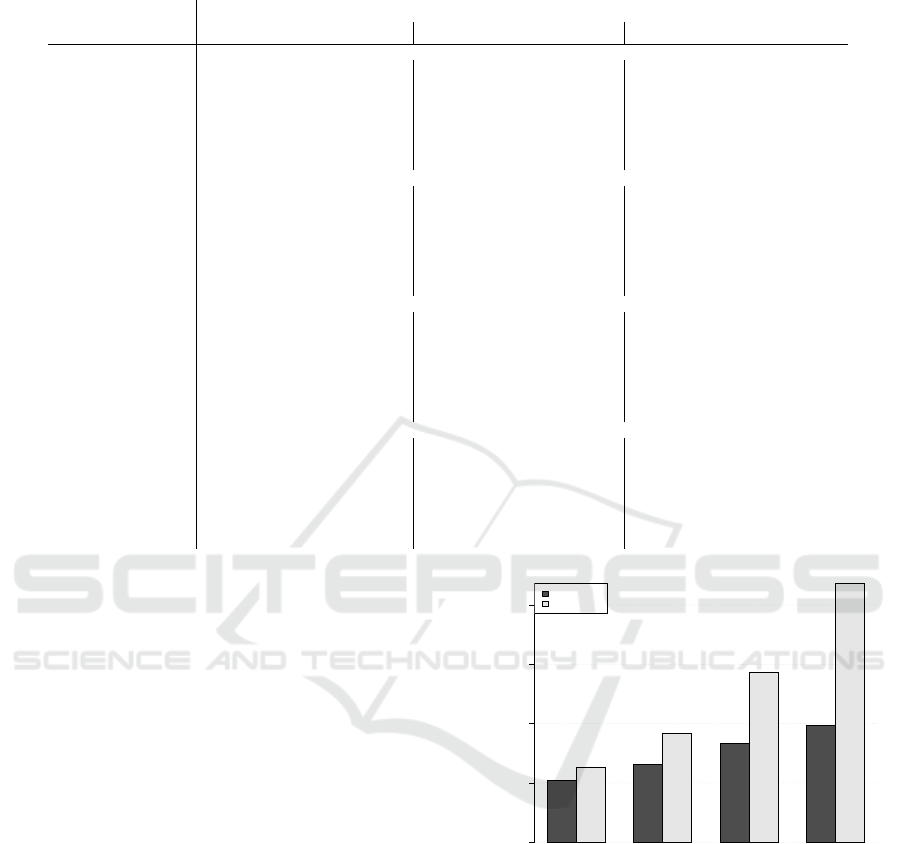
Table 5: Performance measures of pickup models under forecasting horizons, 7, 14, 28 and 56 days out. Carpark: CP1.

Pickup model

MAE sMAPE RMSE

7 14 28 56 7 14 28 56 7 14 28 56

Add-Class-HA 27.93 33.07 39.07 40.06 21.28 24.87 29.10 30.42 36.04 42.99 48.99 50.38

Add-Class-ES 26.42 32.04 41.19 47.09 20.28 24.40 30.73 34.89 34.61 43.15 53.61 59.43

Add-Class-Holt 27.69 36.05 48.63 60.38 21.15 27.89 37.59 45.13 35.57 49.83 67.45 80.54

Add-Class-ARIMA 28.69 34.42 40.06 41.28 22.18 26.26 30.29 31.99 37.11 45.15 51.77 52.07

Add-Class-HW 26.42 32.51 48.78 60.20 20.97 25.83 38.97 46.74 34.81 45.12 64.41 74.97

Add-Class-STL 25.33 31.11 41.04 46.39 19.99 24.18 31.29 35.16 33.73 42.18 53.38 58.38

Add-Class-SARIMA 30.90 45.57 64.61 103.50 24.96 38.11 49.94 72.44 41.96 60.35 84.99 138.37

Add-Advan-HA 27.93 32.95 38.76 39.48 21.28 24.77 28.76 29.94 36.04 42.82 48.79 49.44

Add-Advan-ES 25.68 31.06 38.08 41.65 19.95 23.93 28.52 31.24 33.57 41.14 49.61 52.87

Add-Advan-Holt 27.11 33.71 45.28 59.14 20.56 25.33 32.93 41.95 35.03 45.04 61.50 77.12

Add-Advan-ARIMA 26.49 33.06 41.76 45.01 20.44 25.44 30.96 33.56 34.25 43.31 53.11 60.88

Add-Advan-HW 24.42 30.76 40.63 49.83 19.61 24.64 31.52 38.39 31.97 40.82 53.78 61.15

Add-Advan-STL 24.69 31.32 39.87 49.07 19.58 24.56 30.39 36.77 32.70 40.96 52.23 60.26

Add-Advan-SARIMA 26.05 34.61 47.32 60.92 20.82 27.47 35.80 44.12 33.95 45.26 60.09 76.52

Mult-Class-HA 35.60 56.27 90.72 165.63 25.69 37.13 55.44 93.60 45.78 75.05 126.19 277.68

Mult-Class-ES 35.62 62.58 93.10 175.66 25.68 38.08 56.09 95.51 47.34 100.95 132.91 305.30

Mult-Class-Holt 38.37 74.30 109.87 257.00 26.86 41.64 64.75 103.76 51.24 129.89 158.61 556.16

Mult-Class-ARIMA 34.18 53.01 90.51 147.93 24.97 35.74 56.35 92.28 44.78 71.01 127.40 236.11

Mult-Class-HW 36.60 67.54 147.18 241.73 26.27 40.77 74.69 109.34 48.32 121.63 324.77 404.13

Mult-Class-STL 35.04 58.54 97.35 181.89 25.18 35.77 56.52 97.03 47.04 101.42 152.07 312.20

Mult-Class-SARIMA 30.90 45.57 64.61 103.50 24.96 38.11 49.94 72.44 41.96 60.35 84.99 138.37

Mult-Advan-HA 34.83 52.08 86.58 210.99 25.49 35.74 53.27 71.80 44.47 67.14 121.39 448.30

Mult-Advan-ES 32.56 51.55 91.97 195.98 24.20 34.85 53.32 75.44 41.57 70.53 143.08 333.87

Mult-Advan-Holt 34.39 57.55 119.38 341.33 24.68 36.95 60.72 92.99 46.77 85.66 207.52 649.49

Mult-Advan-ARIMA 32.75 49.01 86.63 173.32 24.63 34.42 54.38 72.92 42.45 65.08 122.94 305.91

Mult-Advan-HW 34.32 52.66 140.92 318.52 24.99 34.42 56.48 84.80 45.00 79.73 442.80 805.13

Mult-Advan-STL 34.71 53.47 130.82 279.73 25.20 34.74 55.84 82.00 46.90 82.27 449.37 825.88

Mult-Advan-SARIMA 33.36 51.64 96.25 217.97 24.22 34.71 54.81 78.87 43.65 70.43 139.45 409.44

additive or multiplicative type. Additive pickup

models seem to have outperformed the multiplica-

tive ones. In general, additive methods are more

robust as they still perform reasonably well for

longer horizons. In contrast, multiplicative meth-

ods seem to perform reasonably well for shorter

horizons, but quickly deteriorate as we move fur-

ther out in the future. Given that multiplicative

variations apply a percentage ratio to the onhand

bookings in order to obtain the ﬁnal arrivals, it

implies that on-hand bookings are crucial to this

calculation; as we attempt to forecast further out

in the future, the underlying onhand bookings are

very low and highly volatile, which results in in-

ﬂated projections.

• Advanced or Classical?

In ﬁgure 3 we compare all variations based on

their classical or advanced type. Both approaches

seem to perform similarly; advanced pickup mod-

els perform marginally better than classical ones,

with the improvement in performance to become

more apparent at longer horizons. There are two

reasons that cause this; ﬁrst, advanced models

use all completed and partially completed book-

ing curves in forecasting, a strategy that more ef-

fectively utilises the short term dynamics of the

h7 h14 h28 h56

Forecast horizon (days)

sMAPE

h7 h14 h28 h56

additive

multiplicative

Figure 2: Comparison of additive versus multiplicative vari-

ations. sMAPE for CP1 under all forecast horizons, 7, 14,

28 and 56 days out.

data as these are unfolding. Second, advanced

pickup models split the forecast horizon down by

reading day and perform a forecast for each read-

ing day separately. Having the data disaggregated

down by reading day prevents the loss of data

that would have been caused from aggregating.

The further out we forecast, the larger is the ag-

gregated bookings-to-come forecast required and

given that in classical pickup this is all estimated

as a whole, leads to lower forecast accuracy.

A Comparative Analysis of Pickup Forecasting Methods for Customer Arrivals in Airport Carparks

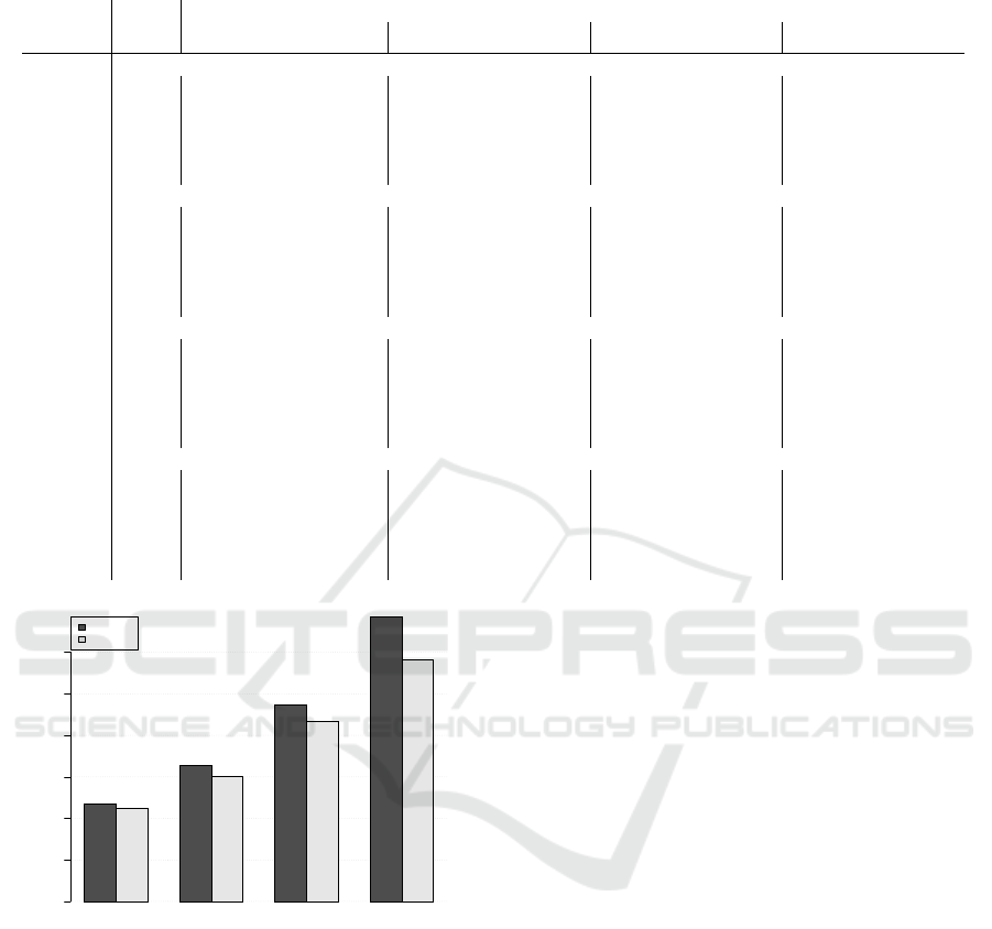
Table 6: Best ﬁve pickup models for each carpark.

Carpark Rank

Days out (h)

7 14 28 56

CP1

1 Add-Advan-HW Add-Advan-ES Add-Advan-HA Add-Advan-HA

2 Add-Advan-STL Add-Advan-HW Add-Advan-ES Add-Class-HA

3 Add-Advan-ES Add-Class-STL Add-Class-HA Add-Class-ARIMA

4 Add-Class-STL Add-Advan-STL Add-Class-ARIMA Add-Advan-ES

5 Add-Class-ES Add-Class-ES Add-Advan-STL Add-Class-STL

CP2

1 Add-Advan-ES Add-Class-ARIMA Add-Advan-ES Add-Class-ARIMA

2 Add-Class-ES Add-Advan-ES Add-Advan-HA Add-Class-HA

3 Add-Class-ARIMA Add-Advan-HA Add-Class-ARIMA Add-Advan-ES

4 Add-Advan-ARIMA Add-Class-HA Add-Class-HA Add-Advan-HA

5 Add-Advan-STL Add-Advan-HW Add-Class-ES Add-Class-ES

CP3

1 Add-Class-SARIMA Add-Advan-ES Add-Advan-ES Add-Class-ARIMA

2 Add-Advan-ES Add-Class-ARIMA Add-Advan-STL Add-Class-HA

3 Mult-Class-SARIMA Add-Advan-ARIMA Add-Advan-HW Add-Advan-ES

4 Add-Class-ES Add-Advan-HA Add-Advan-HA Add-Advan-HA

5 Add-Advan-HW Add-Advan-HW Add-Class-ARIMA Add-Advan-STL

CP4

1 Mult-Advan-SARIMA Add-Advan-ES Add-Advan-ES Add-Advan-ES

2 Add-Advan-STL Add-Advan-STL Add-Advan-STL Add-Advan-STL

3 Add-Advan-ES Add-Advan-ARIMA Add-Advan-HW Add-Advan-HW

4 Add-Advan-HW Add-Advan-HW Add-Advan-ARIMA Add-Class-ES

5 Mult-Class-STL Add-Advan-SARIMA Add-Advan-HA Add-Advan-HA

h7 h14 h28 h56

Forecast horizon (days)

sMAPE

h7 h14 h28 h56

classical

advanced

Figure 3: Comparison of classical versus advanced varia-

tions. sMAPE for CP1 under all forecast horizons, 7, 14, 28

and 56 days out.

• Which Time-series model?

In ﬁgure 4 we test all variations based on their un-

derlying time series model used. For short fore-

casts horizons (h=7, 14) the most sophisticated

models seem to have been the favourites while for

longer horizons (h=28, 56) simpler models have

at least performed as well. More precisely, time

series models like HW, STL and SARIMA per-

formed very well for h = 7, indicating dealing

explicitly with seasonality, as opposed to remov-

ing, is the best approach with regards to short-

term forecasting. As we gradually step into longer

horizons, especially for h = 28, 56, simple his-

torical or weighted averages by day-of-week be-

gin to gain attention. This is because, the further

out we forecast the less the intra-day effects are

and the stronger the weekly seasonality becomes,

which implies that focusing on same days of the

week and applying a simpler forecast on the re-

sulting series gives reasonable forecasts. Note that

ARIMA and SARIMA models variations do ap-

pear among the top ﬁve in most instances but the

computations times, being much higher than the

other models, render them less attractive in prac-

tice.

3.2 Best Overall Pickup Models

Table 6 summarises the best ﬁve winning variations

based on forecast performance, by carpark and by

forecast horizon (as described in section 2.4). Our

study identiﬁed that additive advanced combinations

dominate for both carparks and all forecast horizons;

out of the eighty total instances that make up the top

ﬁve list for all horizons and carparks, only one third

are classical models, while only three instances refer

to multiplicative model variations. STL and HW seem

to be the dominant methods as they most of the times

ranked among the top ﬁve in both carparks and all

ICORES 2016 - 5th International Conference on Operations Research and Enterprise Systems

h7 h14 h28 h56

Forecast horizon (days)

sMAPE

h7 h14 h28 h56

Holt

ARIMA

STL

SARIMA

Figure 4: Comparison of variations based on the underly-

ing time series models. sMAPE for CP1 under all forecast

horizons, 7, 14, 28 and 56 days out.

forecasting horizons. Simpler models such as HA and

ES have also shown to be consistent and performed

well, and for longer horizons they claimed top spots.

4 CONCLUSION

In this paper, we have presented 28 variations of

the pickup method. Experiments were conducted on

reservations data from four airport carparks of a major

airport in UK. The performance of each model vari-

ation was evaluated under three different error mea-

sures and for different forecast horizons, spanning

from 1 week to 8 weeks out. Our study has shown

that the best practice is to use a combination of mod-

els; perhaps a highly sophisticated model for short-

term forecasting and a simple weighted moving aver-

age for longer forecasting.

Our research aims to examine further the role of

the training set in forecast performance. More pre-

cisely, the training set can be of two types; “ﬁxed”

for a pre-determined training size that rolls for-

ward as time progresses and updates accordingly, or

“growing” that increases with time and thus always

uses all the available data. Moreover, already under

progress is the examination of regression forecasting

models which we aim to compare against the best

pickup methods. Regression model variations relate

the total arrivals to the on-hand ones with the possibil-

ity to include other factors such as weekly seasonality,

linear trends or even ﬂight information. Finally, we

are intrigued in exploiting the potential of combining

two or more forecasts to ultimately obtain a more ac-

curate combined forecast.

REFERENCES

Cleveland, R., Cleveland, W., McRae, J., and Terpenning,

I. (1990). Seasonal-trend decomposition procedure

based on loess. Journal of ofﬁcial satistics, 6(1):3–73.

Hyndman, R. and Khandakar, Y. (2007). Automatic time

series forecasting: the forecast package for r. URL

http://www. jstatsoft. org/v27/i03.

Hyndman, R., Koehler, A. B., Ord, J. K., and Snyder, R. D.

(2008). Forecasting with exponential smoothing: the

state space approach. Springer.

Hyndman, R. J., Koehler, A. B., Snyder, R. D., and Grose,

S. (2002). A state space framework for automatic fore-

casting using exponential smoothing methods. inter-

national Journal of Forecasting, 18(3):439–454.

Lee, A. O. (1990). Airline reservations forecasting; prob-

abilistic and statistical models of the booking pro-

cess. PhD thesis, Massachusetts Institute of Technol-

ogy, MIT.

Makridakis, S., Wheelwright, S. C., and Hyndman, R. J.

(2008). Forecasting methods and applications. John

Wiley & Sons.

Papayiannis, A., Johnson, P., Yumashev, D., and Duck,

P. (2013). Continuous-time revenue management in

carparks - part two: Reﬁning the pde. In Proceed-

ings of the 2nd International Conference on Opera-

tions Research and Enterprise Systems, pages 76–81.

ICORES, SciTePress Digital Library.

Papayiannis, A., Johnson, P., Yumashev, D., Howell, S.,

Proudlove, N., and Duck, P. (2012). Continuous-

time revenue management in carparks. In Proceed-

ings of the 1st International Conference on Opera-

tions Research and Enterprise Systems, pages 73–82.

ICORES, SciTePress Digital Library.

olt, S. (1998). Forecasting is difﬁcult–especially if it

refers to the future. In Reservation and Yield Man-

agement Study Group Annual Meeting Proceedings,

Melbourne, Australia. AGIFORS.

Rojas, D. (2006). Revenue management techniques ap-

plied to the parking industry. Master’s thesis, School

of Industrial and Systems Engineering, University of

Florida.

Sa, J. (1987). Reservations forecasting in airline yield man-

agement. Technical report, Flight Transportation Lab-

oratory, Massachusetts Institute of Technology.

Shumway, R. H., Stoffer, D. S., and Stoffer, D. S. (2000).

Time series analysis and its applications: with R ex-

amples. Springer.

Weatherford, L. and P

olt, S. (2002). Better unconstraining

of airline demand data in revenue management sys-

tems for improved forecast accuracy and greater rev-

enues. Journal of Revenue and Pricing Management,

1:234–254.

Weatherford, L. R. and Kimes, S. E. (2003). A comparison

of forecasting methods for hotel revenue management.

International Journal of Forecasting, 19(3):401–415.

Weatherford, L. R., Kimes, S. E., and Scott, D. A. (2001).

Forecasting for hotel revenue management: Testing

aggregation against disaggregation. The Cornell Ho-

A Comparative Analysis of Pickup Forecasting Methods for Customer Arrivals in Airport Carparks

tel and Restaurant Administration Quarterly, 4(4):53–

64.

Wickham, R. R. (1995). Evaluation of forecasting tech-

niques for short-term demand of air transportation.

Master’s thesis, Massachusetts Institute of Technol-

ogy, Dept. of Aeronautics & Astronautics, Flight

Transportation Laboratory, Cambridge, MA.

Zakhary, A., Neamat, E. G., and Amir, F. A. (2008). A com-

parative study of the pickup method and its variations

using a simulated hotel reservation data. ICGST In-

ternational Journal on Artiﬁcial Intelligence and Ma-

chine Learning, pages 15–21.

ICORES 2016 - 5th International Conference on Operations Research and Enterprise Systems